Summary
The following is a demonstration of multiple linear modeling using a canned dataset in R. The demo includes some recoding, exploratory data visualization, a discussion of multicolinearity and model selection, and residual analysis.
The “mtcars” dataset was extracted from the 1974 Motor Trend US magazine, and comprises fuel consumption and 10 aspects of automobile design and performance for 32 automobiles (1973–74 models) (R Package: datasets, Version 3.4.1).
library(datasets)
str(mtcars)
## 'data.frame':	32 obs. of  11 variables:
##  $ mpg : num  21 21 22.8 21.4 18.7 18.1 14.3 24.4 22.8 19.2 ...
##  $ cyl : Factor w/ 3 levels "4cyl","6cyl",..: 2 2 1 2 3 2 3 1 1 2 ...
##  $ disp: num  160 160 108 258 360 ...
##  $ hp  : num  110 110 93 110 175 105 245 62 95 123 ...
##  $ drat: num  3.9 3.9 3.85 3.08 3.15 2.76 3.21 3.69 3.92 3.92 ...
##  $ wt  : num  2.62 2.88 2.32 3.21 3.44 ...
##  $ qsec: num  16.5 17 18.6 19.4 17 ...
##  $ vs  : Factor w/ 3 levels "3","4","5": 1 1 2 2 1 2 1 2 2 2 ...
##  $ am  : Factor w/ 2 levels "Automatic","Manual": 2 2 2 1 1 1 1 1 1 1 ...
##  $ gear: Factor w/ 3 levels "3","4","5": 2 2 2 1 1 1 1 2 2 2 ...
##  $ carb: Factor w/ 8 levels "1","2","3","4",..: 4 4 1 1 2 1 4 2 2 4 ...
Does the distance a car can drive on a gallon of gas (MPG) depend on whether or not the car has an automatic or manual transmission? We can quantify the MPG difference in manual vs. automatic transmission vehicles, and we can do so while accounting for other confounding variables. I’ll show that transmission type does correspond to a significant MPG difference, but when accounting for the vehicles weight, horsepower, and number of cylinders, the transmission effect goes away.
Data cleaning and preparation
A quick glance at the data shows that all variables are coded and stored numerically. Categorical variables must be recoded as factors.
mtcars$am<-factor(mtcars$am)
levels(mtcars$am)<-c("Automatic", "Manual")
mtcars$cyl<-factor(mtcars$cyl)
levels(mtcars$cyl)<-c("4cyl", "6cyl", "8cyl")
mtcars$vs<-factor(mtcars$vs)
levels(mtcars$vs)<-c("V-shape", "Straight")
mtcars$gear<-factor(mtcars$gear)
levels(mtcars$vs)<-c("3", "4", "5")
mtcars$carb<-factor(mtcars$carb)
levels(mtcars$carb)<-c("1", "2", "3", "4", "5", "6", "7", "8")
Miles per Gallon vs. Transmission Type
summary(mtcars$mpg)
##    Min. 1st Qu.  Median    Mean 3rd Qu.    Max.
##   10.40   15.43   19.20   20.09   22.80   33.90
table(mtcars$am)
##
## Automatic    Manual
##        19        13
The milage of the 32 cars in the dataset range from 10.4 to 33.9, with an average MPG of 20.1. Nineteen of these cars have an automatic transmission and thirteen are manual.
boxplot(mpg~am, data=mtcars, ylab="Miles Per Gallon", main="MPG by Transmission Type", col="pink")
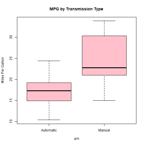
The side-by-side box plot above demonstrates an obvious variation in milage when comparing manual to automatic transmission cars.
t.test(mpg~am, data=mtcars)
##
## 	Welch Two Sample t-test
##
## data:  mpg by am
## t = -3.7671, df = 18.332, p-value = 0.001374
## alternative hypothesis: true difference in means between group Automatic and group Manual is not equal to 0
## 95 percent confidence interval:
##  -11.280194  -3.209684
## sample estimates:
## mean in group Automatic    mean in group Manual
##                17.14737                24.39231
Indeed, we can infer from the t-test above that mileage is related to transmission type. The difference in means (7.24 MPG) is large enough to conclude that there is very little chance (p = .001) that the observed difference is likely to occur by noise in the data alone (c.f., ‘Demo: Statistical Inference’ in this portfolio). Based on bivariate statistics alone, we would reject the null hypothesis and conclude that manual transmissions get better gas mileage (in 1974 at least).
To fully assess whether transmission type is a significant determinant of gas mileage, however, we must account for possible confounding variables. That is, transmission type may be related to other factors, such as engine size, weight, or horsepower, each of which may better explain variation in gas mileage.
Multiple Regression Analysis
Standard OLS linear regression allows for testing the effect of transmission on mileage while holding other variables constant. Further, analysis of model variance allows for understanding the best model fit, and a discussion of the model’s residuals will show us if the model is an appropriate analytical tool.
In fact, every other variable included in the dataset has a statistically significant relationship to a car’s MPG (not shown). Below, I regress each variable on gas mileage simultaneously, so that we can see the effect of each, holding each other constant. Note: I omit the car’s 1/4 mile time because this variable is, like MPG, a performance measure, so it would seem likely that they are spuriously correlated; I also omit the variable gear, because gear number is correlated with transmission type by design.
fullmodel<-lm(mpg~am+cyl+disp+hp+drat+wt+vs+carb, data=mtcars); # i.e, full without qsec and gears
summary(fullmodel)
##
## Call:
## lm(formula = mpg ~ am + cyl + disp + hp + drat + wt + vs + carb,
##     data = mtcars)
##
## Residuals:
##     Min      1Q  Median      3Q     Max
## -3.7086 -1.4119  0.0302  0.7624  4.3994
##
## Coefficients:
##             Estimate Std. Error t value Pr(>|t|)
## (Intercept) 28.86269   10.94309   2.638   0.0167 *
## amManual     1.60639    2.04356   0.786   0.4421
## cyl6cyl     -3.14936    2.53987  -1.240   0.2309
## cyl8cyl     -2.32360    5.09121  -0.456   0.6536
## disp         0.03556    0.02660   1.337   0.1980
## hp          -0.06604    0.03102  -2.129   0.0473 *
## drat         1.50319    2.23163   0.674   0.5091
## wt          -4.23798    2.04813  -2.069   0.0532 .
## vs4          2.38609    2.36209   1.010   0.3258
## carb2       -0.45802    1.65845  -0.276   0.7856
## carb3        3.58575    3.88249   0.924   0.3679
## carb4        1.10296    3.42655   0.322   0.7512
## carb5        5.07957    5.60594   0.906   0.3769
## carb6        8.08435    7.32199   1.104   0.2841
## ---
## Signif. codes:  0 '***' 0.001 '**' 0.01 '*' 0.05 '.' 0.1 ' ' 1
##
## Residual standard error: 2.642 on 18 degrees of freedom
## Multiple R-squared:  0.8884,	Adjusted R-squared:  0.8079
## F-statistic: 11.03 on 13 and 18 DF,  p-value: 4.8e-06
The full model summary shows us that, controlling for other factors, the effect of transmission type on gas mileage all but dissapears. The effect is still positive (manual transmission cars get a mean 1.6 MPGs better than automatics, instead of 7.24), but it is no longer statistically significant (p = .44), and so we cannot conclude that the difference is not due to random chance. In fact, in the full model, we see very little statistically significant correlates to mpg. Only horsepower is signficantly related. A one unit increase in horsepower leads to a decrease in .06 miles to the gallon, holding every other variable constant.
Model Selection
It should not be surprising that we see few significant predictors of mpg, however, because our n is so small; we have a tiny number of cases for each indpendent variable. We can look for a better explanatory model whose least squares minimize the variance. The R function step(), below, calculates the variances of models of multiple smaller combinations of variables included in our original full model.
best<-step(fullmodel, direction="both"); # hidden to save space
summary(best)
##
## Call:
## lm(formula = mpg ~ am + cyl + hp + wt, data = mtcars)
##
## Residuals:
##     Min      1Q  Median      3Q     Max
## -3.9387 -1.2560 -0.4013  1.1253  5.0513
##
## Coefficients:
##             Estimate Std. Error t value Pr(>|t|)
## (Intercept) 33.70832    2.60489  12.940 7.73e-13 ***
## amManual     1.80921    1.39630   1.296  0.20646
## cyl6cyl     -3.03134    1.40728  -2.154  0.04068 *
## cyl8cyl     -2.16368    2.28425  -0.947  0.35225
## hp          -0.03211    0.01369  -2.345  0.02693 *
## wt          -2.49683    0.88559  -2.819  0.00908 **
## ---
## Signif. codes:  0 '***' 0.001 '**' 0.01 '*' 0.05 '.' 0.1 ' ' 1
##
## Residual standard error: 2.41 on 26 degrees of freedom
## Multiple R-squared:  0.8659,	Adjusted R-squared:  0.8401
## F-statistic: 33.57 on 5 and 26 DF,  p-value: 1.506e-10
R’s step() function returns the model that says (which model represents the least residual variance): Gas milage is a function of transmission type, number of cylinders, horsepower, and the vehicle’s weight. Compared to the full model, we see that vehicle weight now seems to be the strongest predictor of gas mileage, while horsepower, and number of cylinders (specifically the difference between 4 and 6 cylinders) also have significant effects. Transmission type, although it is included in our model, remains statistically insignificant, and so we cannot reject the null hypothesis: we cannot conclude that manual transmission vehicles get better gas mileage.
Residual Diagnostics
par(mfrow=c(2,2))
plot(best)
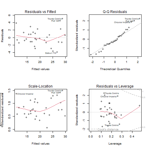
Residuals appear random and independent, normally distributed, and have no outliers.
Conclusion
Althought transmission type is related to gas mileage at the bivariate level, controlling for number of cylinders, vehicle’s weight, and horsepower, the significant effect of transmission type goes away. We cannot be sure that manual transmission cars get better gas mileage than automatics. However, because the number of vehicles in the sample is low, our model does not contain much statistical power, and multiple regression may not be an ideal method of analysis given the sample size. Further research should seek to obtain a larger sample size (ideally 80+ cars).
Appendix
The dataset includes 32 observations and the following variables:
mpg Miles/(US) gallon cyl Number of cylinders disp Displacement (cu.in.) hp Gross horsepower drat Rear axle ratio wt Weight (1000 lbs) qsec 1/4 mile time vs V/S am Transmission (0 = automatic, 1 = manual) gear Number of forward gears carb Number of carburetors (R Package: datasets, Version 3.4.1)
Other correlations
# Vehicle weight
with(mtcars, cor.test(mpg, wt))[4:3]
## $estimate
##        cor
## -0.8676594
##
## $p.value
## [1] 1.293959e-10
# Horsepower
with(mtcars, cor.test(mpg, hp))[4:3]
## $estimate
##        cor
## -0.7761684
##
## $p.value
## [1] 1.787835e-07
# Displacement
with(mtcars, cor.test(mpg, disp))[4:3]
## $estimate
##        cor
## -0.8475514
##
## $p.value
## [1] 9.380327e-10
# Rear axle ratio
with(mtcars, cor.test(mpg, drat))[4:3]
## $estimate
##       cor
## 0.6811719
##
## $p.value
## [1] 1.77624e-05
# 1/4 mile time
with(mtcars, cor.test(mpg, qsec))[4:3]
## $estimate
##      cor
## 0.418684
##
## $p.value
## [1] 0.01708199
# V/S (shape of engine)
t.test(mpg~vs, data=mtcars)[3]
## $p.value
## [1] 0.0001098368
# Number of cylinders
summary(lm(mpg~cyl, data=mtcars))$coef
##               Estimate Std. Error   t value     Pr(>|t|)
## (Intercept)  26.663636  0.9718008 27.437347 2.688358e-22
## cyl6cyl      -6.920779  1.5583482 -4.441099 1.194696e-04
## cyl8cyl     -11.563636  1.2986235 -8.904534 8.568209e-10
# Number of gears
summary(lm(mpg~gear, data=mtcars))$coef
##              Estimate Std. Error   t value     Pr(>|t|)
## (Intercept) 16.106667   1.215611 13.249852 7.867272e-14
## gear4        8.426667   1.823417  4.621361 7.257382e-05
## gear5        5.273333   2.431222  2.169005 3.842222e-02
# Number of carburetors
summary(lm(mpg~carb, data=mtcars))$coef
##               Estimate Std. Error   t value     Pr(>|t|)
## (Intercept)  25.342857   1.853844 13.670438 2.214664e-13
## carb2        -2.942857   2.417117 -1.217507 2.343463e-01
## carb3        -9.042857   3.384640 -2.671734 1.284993e-02
## carb4        -9.552857   2.417117 -3.952170 5.295477e-04
## carb5        -5.642857   5.243462 -1.076170 2.917362e-01
## carb6       -10.342857   5.243462 -1.972524 5.927269e-02