Summary
This project demonstrates 1. Visualization using Tableau, and 2. Getting and cleaning a large dataset.
One of my pet research questions is: Why and where do (some) occupations agglomerate? Or, what kinds of places attract certain kinds of jobs? Arts occupations are interesting becuase the rewards are often reputational rather than economic, and the benefits of place include the presence of markets, scenes, and the status associated with a place itself. That is, artists might locate where the action is, not where there are “jobs” per se. On the other hand, a decade or so ago the “creative city” mantra made attracting artists an urban planning priority.
In this demonstration, we’ll view artist location patterns by discipline, including their ‘relative’ metro distributions. In the long run, I’ll want to use this data to see if the pandemic had any real effect on occupational diffusion.
Visualization Using Tableau
In the dashboard embedded here, users can search by artistic discipline, and order by Metro art population or relative metro arts population (LQ).
For a more responsive dashboard, please visit my Tableau public viz here: Where do Artists Live?
Getting and Cleaning a Large Dataset
The ACS is a 1% survey of the U.S. population conducted annually by the U.S. Census Bureau as a complement to the decennial census. The ACS adds depth and a broader range of demographic, housing and economic data that the 9-question census cannot capture.
The 1% “microsamples” are available in 5-year - or 5% - datasets, which provide more stable population estimates. The 2022 5-year ACS, for example, is actually 5, 1-year, 1% samples combined, from 2018-2022, but include weights only interpretable for the 5 year set.
Data are available online at census.gov, or at the more user friendly IPUMS website (https://usa.ipums.org/usa/). IPUMS stands for Integrated Public Use Microsample Series. Users can select the samples and the columns of data they want to analyze, and find all the codebooks, questionaires and other documentation there. Getting Data from IPUMS requires permission. They vet your request and then provide a downloadable zip file, usually within hours.
Beware of large file sizes! Each 1% of the U.S. population is about 3.5 million cases. A 5-year dataset will contain close to 18 million rows.
ACS_2022<-read.csv("ACS PUMS/usa_00011.csv")
str(ACS_2022)
## 'data.frame':	15721123 obs. of  30 variables:
##  $ OCC       : int  0 0 0 0 0 0 0 0 0 0 ...
##  $ MET2013   : int  0 0 12580 12580 0 12580 31140 0 0 0 ...
##  $ YEAR      : int  2022 2022 2022 2022 2022 2022 2022 2022 2022 2022 ...
##  $ MULTYEAR  : int  2018 2018 2019 2019 2018 2019 2020 2022 2018 2019 ...
##  $ SAMPLE    : int  202203 202203 202203 202203 202203 202203 202203 202203 202203 202203 ...
##  $ SERIAL    : int  3166637 2072182 2876368 2891675 11876 2899243 2671413 2441410 1359389 5706277 ...
##  $ HHWT      : num  9 5 3 112 13 17 4 13 12 6 ...
##  $ DENSITY   : num  123 172 452 2316 232 ...
##  $ MET2013ERR: int  0 0 3 3 0 3 3 0 0 0 ...
##  $ METPOP10  : int  126933 50687 2710489 2710489 106154 2710489 1235708 49519 46809 97991 ...
##  $ OWNERSHP  : int  1 1 0 2 1 1 1 0 1 1 ...
##  $ OWNERSHPD : int  13 13 0 22 12 13 13 0 12 12 ...
##  $ HHINCOME  : int  70144 77158 9999999 122285 68741 133193 5439 9999999 107554 24113 ...
##  $ PERWT     : num  12 10 3 106 12 18 1 13 16 6 ...
##  $ SEX       : int  2 2 1 2 2 1 1 1 1 1 ...
##  $ AGE       : int  14 3 90 12 65 16 2 46 9 85 ...
##  $ RACE      : int  1 1 2 2 1 1 7 2 1 1 ...
##  $ RACED     : int  100 100 200 200 100 100 700 200 100 100 ...
##  $ HISPAN    : int  0 0 0 0 0 0 0 0 0 0 ...
##  $ HISPAND   : int  0 0 0 0 0 0 0 0 0 0 ...
##  $ EDUC      : int  3 0 10 2 7 4 0 6 1 6 ...
##  $ EDUCD     : int  30 2 101 23 71 40 1 63 17 65 ...
##  $ DEGFIELD  : int  0 0 61 0 0 0 0 0 0 0 ...
##  $ DEGFIELDD : int  0 0 6108 0 0 0 0 0 0 0 ...
##  $ DEGFIELD2 : int  0 0 0 0 0 0 0 0 0 0 ...
##  $ DEGFIELD2D: int  0 0 0 0 0 0 0 0 0 0 ...
##  $ INCTOT    : int  9999999 9999999 10334 9999999 33342 0 9999999 0 9999999 24113 ...
##  $ SEI       : int  0 0 0 0 0 0 0 0 0 0 ...
##  $ Metro     : chr  "Not in identifiable area" "Not in identifiable area" "Baltimore-Columbia-Towson, MD" "Baltimore-Columbia-Towson, MD" ...
##  $ Occupation: chr  "N/A (not applicable)" "N/A (not applicable)" "N/A (not applicable)" "N/A (not applicable)" ...
I Asked for a dozen or so columns, plus IPUMS gives you some extras, like DEGFIELDD (which is a detailed code of DEGFIELD (degree field)). Make sure you ask for Person- and/or Household- weights, depending on what type of analysis you want to do.
In this project I’m interested in what types of occupations tend to agglomerate (or are diffuse) in particular places. Or, perhaps, what kind of places attract particular occupations. In the long run, I’ll want to use this data to see if the pandemic had any real effect on occupational diffusion.
Data Preparation
Because I’m interested in Metro Areas and Occupations, the first step will be to add the labels to these codes. Rather than manually recoding these variables however (There are 282 Metro codes and 500+ occupation codes), we’ll recode by merging a list.
The trick is to copy/paste the code book to a excel file, save as a .csv, and then merge on the numeric code.
Here is what the labels look like in the codebook:
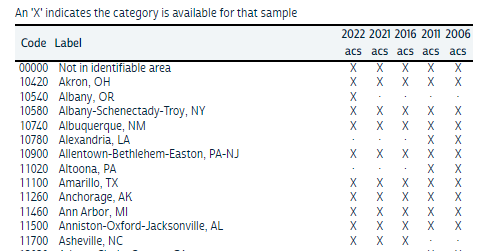
After copy/pasting the first two columns and saving as a .csv…
metro_labels<-read.csv("ACS PUMS/MET2013_Labels.csv")
str(metro_labels)
## 'data.frame':	312 obs. of  2 variables:
##  $ MET2013: int  0 10420 10540 10580 10740 10780 10900 11020 11100 11260 ...
##  $ Metro  : chr  "Not in identifiable area" "Akron, OH" "Albany, OR" "Albany-Schenectady-Troy, NY" ...
ACS_2022<-merge(ACS_2022, metro_labels, by = "MET2013", all.x=TRUE)
Do the same for occupation labels.
occ_labels<-read.csv("ACS PUMS/Occ_Names.csv")
ACS_2022<-merge(ACS_2022, occ_labels, by="OCC", all.x=TRUE)
Where are the artists (in the data)?
The OCC (Occupation) code for “Artists and Related Workers” is 2600
sum(ACS_2022$OCC==2600)
## [1] 17883
There are 17883 cases of people who claimed Artist as their primary occupation in the 5 1% microsample surveys, 2018-2022…
sum(ACS_2022$PERWT[ACS_2022$OCC==2600])
## [1] 354607
… which theoretically represent (i.e., with person weights) 354,607 artists.
But there are many arts or arts-adjacent occupations, including:
2600: Artists and Related Workers 2631: Commercial and Industrial Designers 2632: Fashion Designers 2634: Graphic Designers 2635: Interior Designers 2640: Other Designers 2700: Actors 2710: Producers and Directors 2740: Dancers and Choreographers 2751: Music Directors and Composers 2752: Musicians and Singers 2850: Writers and Authors 2910: Photographers
Not all arts fields are the same, and each may have a different relationship to place. The film industry is famously centered around Hollywood, while writers and/or photographers might not have a distinct occupational center. So lets include all the disciplines in our study and you can note the differences if you see any.
Aggregate arts occupation populations for each Metro area.
First, I subset our arts occupations: Rows that have a specific OCC code, and all columns (for now).
Art_occ_dt<-ACS_2022[ACS_2022$OCC %in% c(2600,2631,2632,2634,2635,2640,2700,2710,
					 2740,2751,2752,2850,2910),]
Next, I aggregate by summing each occupation within each Metro, being sure to use the per/person weights provided in the dataset (Note: the ACS weights are calculated for the 5-year dataset and should only be used as such).
I will take the liberty of dividing the occupation categories as I want. For example, I’m grouping musicians, singers and composers, and I’m separating fashion designers and graphic designers from “other designers”.
library(dplyr)

Arts_agg<-Art_occ_dt %>%
	group_by(Metro) %>%
	summarize(
		Artists = sum(PERWT[OCC==2600], na.rm=TRUE),
		Graphic_Designers = sum(PERWT[OCC==2634], na.rm=TRUE),
		Fashion_Designers = sum(PERWT[OCC==2632], na.rm=TRUE),
		Other_Designers = sum(PERWT[OCC %in% c(2631,2633,2635,2640)], na.rm=TRUE),
		Musicians = sum(PERWT[OCC %in% c(2751,2752)], na.rm=TRUE),
		Writers = sum(PERWT[OCC==2850], na.rm=TRUE),
		Photographers = sum(PERWT[OCC==2910], na.rm=TRUE),
		Dancers_Chors = sum(PERWT[OCC==2740], na.rm=TRUE),
		Actors = sum(PERWT[OCC==2700], na.rm=TRUE),
		Producers_Dirs = sum(PERWT[OCC==2710], na.rm=TRUE)
	)
To see whether or not a metro artist population is not simply a function of that city’s size, I construct a relative measure that accounts for Metro size. I calculate a Location Quotient (LQ) as the relative share of each art occupation in a city compared to their portion of the national work force. That is: LQ = (local occupation population/local total labor force)/(national occupation population/national total labor force).
The L.Q. is easily interpreted as the [X-local arts population] LQtimes the national average. For example, there are six times the number or artists in Santa Fe, compared to the average U.S. metro area.
# Calculate National Total Labor Force
NAT_TOT_LABOR_FORCE<-sum(ACS_2022$PERWT[ACS_2022$OCC>0])
# OCC>0 ensures that we're comparing artists to others in the labor force (i.e., has an occupational code), not the whole population.

# Calculate Metro labor force (a sum of workforce in each Metro)
metro_labor_force<-ACS_2022 %>%
	filter(OCC>0) %>%
	group_by(Metro) %>%
	summarize(Metro_labor_force = sum(PERWT, na.rm=TRUE))

# Include Metro labor force in our aggregated table
Arts_agg<-merge(metro_labor_force,
		Arts_agg,
		by = "Metro", all.x=TRUE)

# We can get the national artist' labor force by summing the local artists in each Metro.
Arts_relative<-Arts_agg %>%
	mutate(Artists = (Artists/Metro_labor_force)/(sum(Artists)/NAT_TOT_LABOR_FORCE),
	       Graphic_Designers = (Graphic_Designers/Metro_labor_force)/(sum(Graphic_Designers)/NAT_TOT_LABOR_FORCE),
	       Fashion_Designers = (Fashion_Designers/Metro_labor_force)/(sum(Fashion_Designers)/NAT_TOT_LABOR_FORCE),
	       Other_Designers = (Other_Designers/Metro_labor_force)/(sum(Other_Designers)/NAT_TOT_LABOR_FORCE),
	       Musicians = (Musicians/Metro_labor_force)/(sum(Musicians)/NAT_TOT_LABOR_FORCE),
	       Writers = (Writers/Metro_labor_force)/(sum(Writers)/NAT_TOT_LABOR_FORCE),
	       Photographers = (Photographers/Metro_labor_force)/(sum(Photographers)/NAT_TOT_LABOR_FORCE),
	       Dancers_Chors = (Dancers_Chors/Metro_labor_force)/(sum(Dancers_Chors)/NAT_TOT_LABOR_FORCE),
	       Actors = (Actors/Metro_labor_force)/(sum(Actors)/NAT_TOT_LABOR_FORCE),
	       Producers_Dirs = (Producers_Dirs/Metro_labor_force)/(sum(Producers_Dirs)/NAT_TOT_LABOR_FORCE)
	)
Combine the LQs and the local arts populations
Arts_all<-merge(Arts_agg,
		Arts_relative,
		by = "Metro", all.x=TRUE)
Save the file to import to Tableau
setwd("C:/Dat_Sci/Data Projects/ACS_Where_Arts")
write.csv(Arts_all, "Arts_all.csv")