Part II: Inferential Data Analysis
Summary
In part one I discussed the Law of Large Numbers and the Central Limit Theorem as the basis for statistical inference. That is, because of the normality of sample statistics, we can use the properties of the normal distribution to test relationships between variables. When n is relatively small, however, we can still use the assumption that sample statistics are normally distributed, but we need to figure more room for error in our estimates, hence we can use the t distribution (which approximates a normal distribution as n increases). In this demo, I will use t tests to examine if (and how) tooth growth varies by taking a supplement and by the size of its dose.
library(datasets)
str(ToothGrowth)
## 'data.frame':	60 obs. of  3 variables:
##  $ len : num  4.2 11.5 7.3 5.8 6.4 10 11.2 11.2 5.2 7 ...
##  $ supp: Factor w/ 2 levels "OJ","VC": 2 2 2 2 2 2 2 2 2 2 ...
##  $ dose: num  0.5 0.5 0.5 0.5 0.5 0.5 0.5 0.5 0.5 0.5 ...
Our dataset contains only 60 observations; 30 for each supplement (OJ, and VC) and 20 for each dose size (.5, 1, and 2). There are only 10 observations in each dose-supplement category.
Summary of the Data
summary(ToothGrowth$len)
##    Min. 1st Qu.  Median    Mean 3rd Qu.    Max.
##    4.20   13.07   19.25   18.81   25.27   33.90
In this dataset, tooth length varies widely, from 4.2 to 33.9, but does that variation depend on the supplement given and the size of the dose?
# Table means toothgrowth by supplement
with(ToothGrowth, tapply(len, supp, mean))
##       OJ       VC
## 20.66333 16.96333
# Table tooth growth by dose size
with(ToothGrowth, tapply(len, dose, mean))
##    0.5      1      2
## 10.605 19.735 26.100
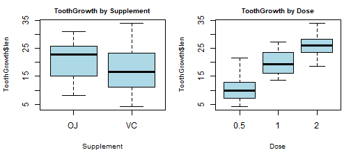
“OJ” is associated with a higher average length than “VC” (mean=20.66 vs. 16.96), but “VC” produces more extreme values on the lower and higher ends of the distribution. The means of tooth length increase for each increase in dose. We can visualize these data using boxplots.
# Side by side box plots
par(mfrow=c(1,2), mar=c(4,4,2,1))
boxplot(ToothGrowth$len~ToothGrowth$supp, col="lightblue",
main="ToothGrowth by Supplement", cex.main=.8, xlab="Supplement", cex.lab=.8)
boxplot(ToothGrowth$len~ToothGrowth$dose, col="lightblue",
main="ToothGrowth by Dose", cex.main=.8, xlab="Dose", cex.lab=.8)
Means Comparisons using T-tests
We can test whether or not the observed differences are due to random chance by determining the probability of those differences using t-tests. The following set of tests make use of the two-sample t.test function in R. We will set alpha = to .05 (the standard default), so we will reject the null hypothesis (that the distributions are equal) if p-values are <.05 for two-tailed tests. That is, we conclude that the relationship is statistically significant if there is a less than 5% probability that the difference is due to chance.
Supplement
Hypothesis 1 (Ha): Tooth length differs depending on the supplement provided. (H0: there is no difference)
oj_len<-ToothGrowth$len[ToothGrowth$supp=="OJ"]
vc_len<-ToothGrowth$len[ToothGrowth$supp=="VC"]
t.test(oj_len, vc_len)
##
## 	Welch Two Sample t-test
##
## data:  oj_len and vc_len
## t = 1.9153, df = 55.309, p-value = 0.06063
## alternative hypothesis: true difference in means is not equal to 0
## 95 percent confidence interval:
##  -0.1710156  7.5710156
## sample estimates:
## mean of x mean of y
##  20.66333  16.96333
The output provides several useful statistics. Notably, it tells us that we are testing the difference between the means 20.66 and 16.96, given the number of observations and the variances of each. The test statistic, 1.92 is the standard error under the t-distribution with 55.3 degrees of freedom. Within our 95% confidence interval (setting alpha = 0.05), the difference in means is not enough standard deviations away to safely reject the null hypothesis (it crosses zero). The p-value is 0.06, which tells us that we can expect to observe as much difference or more in our distributions due to random noise alone about six out of 100 times. Thus, we cannot conclude that the relationship is statistically significant, and so we cannot reject the null hypothesis (given alpha = 0.05).
Now lets visualize by graphing our t-test distribution next to the difference in means.
library(ggplot2)
t_test_result <- t.test(oj_len, vc_len)
t_stat <- t_test_result$statistic
df <- t_test_result$parameter

# Create a sequence of t-values for the t-distribution
t_vals <- seq(-5, 5, length = 1000)
t_dist <- dt(t_vals, df = df)

# Plot the t-distribution
ggplot(data.frame(t_vals, t_dist), aes(x = t_vals, y = t_dist)) +
	geom_line(color = "blue", linetype = "dashed", size = 1.2) + # T-distribution
	geom_vline(xintercept = t_stat, color = "red", linetype = "solid", size = 1.2) + # Observed t-statistic
	geom_vline(xintercept = 0, linetype = "dotted", color = "black", size = 1) + # Line at t=0
	labs(title = "Observed t-statistic vs. Theoretical T-distribution",
	     x = "t-value",
	     y = "Density") +
	theme_minimal() +
	annotate("text", x = t_stat + 0.5, y = max(t_dist) * 0.8,
		 label = paste("t =", round(t_stat, 2)), color = "red", size = 4)
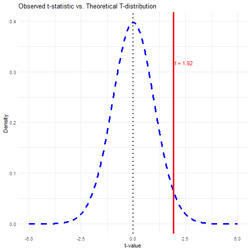
In the graphic illustration, the test statistic, 1.92, is the difference in means standardized by the standard error. i.e., the means are 1.92 standard errors apart, which is not far apart enough to conclude that the difference is not found by chance.
Dose
Hypothesis 2 (Ha): Tooth length depends on the size of the dose (of either supplement). (H0: There is no difference between dose levels). Because the our data show us that mean tooth length increases when we increase the dose, we might use a one.tailed test, hypothesizing that increase in dose leads to increase in tooth growth. But I will opt for the two-sided test, which will provide a more conservative estimate, allowing for the possibility that dose size is associated with decreasing tooth size (albiet unexpected).
with(ToothGrowth, t.test(len[dose==1], len[dose==.5]))
##
## 	Welch Two Sample t-test
##
## data:  len[dose == 1] and len[dose == 0.5]
## t = 6.4766, df = 37.986, p-value = 1.268e-07
## alternative hypothesis: true difference in means is not equal to 0
## 95 percent confidence interval:
##   6.276219 11.983781
## sample estimates:
## mean of x mean of y
##    19.735    10.605
In the first test, we compare a dose of .5 to a dose of 1. The mean tooth lengths are 10.6 and 19.7 respectively. Notably, we observe a p-value of 0.00000012, which represents the probability that the difference in means is due to random chance if the null hypothesis is actually true. The very small p-value suggests that the result would be highly unlikely under the null hypothesis.
with(ToothGrowth, t.test(len[dose==2], len[dose==1]))$p.value
## [1] 1.90643e-05
In the second test (only the p-value is shown), we compare tooth length under a dose of 1 (mean = 19.7) to tooth length under a dose of 2 (mean = 26.1). Again, the p-value is a very small number, indicating very little probability that the difference could be due to chance. In both cases we can safely reject the null hypothesis and conclude that tooth length is strongly associated with the size of dose (of whatever supplement) that is given.
3-way Means Comparisons
Finally, although tooth length does not differ by supplement, we may ask whether or not different doses within supplements produce a difference. The means of supplement-dose categories are tabled below.
means<-xtabs(len/10~supp+dose, data=ToothGrowth)
knitr::kable(means, caption="Tooth Length Means for Supplement and Dose")
Table: Tooth Length Means for Supplement and Dose
| 0.5 | 1 | 2 | |
|---|---|---|---|
| OJ | 13.23 | 22.70 | 26.06 |
| VC | 7.98 | 16.77 | 26.14 |
It may be that tooth length actually does vary by supplement, until we reach high doses.
Hypothesis 3 (Ha): The non-difference in the effect of supplement (see Hypothesis 1) may be explained by the size of the dose.
First, we will test if there is a tooth length difference by supplement for those given a low dose. The means (OJ = 13.23, VC = 7.98) appear different, but the number of observations is also much smaller (only 10 for each category), so now our test must figure-in more chance of random error. In the following tests, I report only p-values to save space.
low<-ToothGrowth[ToothGrowth$dose==.5,]
with(low, t.test(len[supp=="OJ"], len[supp=="VC"]))$p.value
## [1] 0.006358607
Although there are only 15 degrees of freedom (lots of room for error), our test returns a p-value of 0.006, which is less than .05. We can reject the null hypothesis that there is no difference between OJ and VC at low doses.
mid<-ToothGrowth[ToothGrowth$dose==1,]
with(mid, t.test(len[supp=="OJ"], len[supp=="VC"]))$p.value
## [1] 0.001038376
The same pattern holds true for medium doses as well.
high<-ToothGrowth[ToothGrowth$dose==2,]
with(high, t.test(len[supp=="OJ"], len[supp=="VC"]))$p.value
## [1] 0.9638516
But not for high doses.
Conclusion
Variation in tooth length is related to the size of given dose of supplement. The greater the dose, the greater the tooth length (Hyp 2). Tooth length is also related to the type of supplement, but not at all dose sizes (Hyp 3). The tests that we conducted made use of properties associated with the central limit theorem and its assumption of normally distributed sample means. Although the ns were relatively small in the tests conducted, t.tests (using the t distribution) allow for greater random chance associated with smaller sample sizes.