Part I: Simulation

Summary

The simulation and discussion below illustrate the Law of Large Numbers (LLN) and the Central Limit Theorem (CLT) in action. The LLN states that as n increases, statistical estimates approach the true population’s value . The CLT states that as n increases, the averages of variables become normally distributed (despite the shape of the original distribution). For distributions that are not normal, as n increases, the sample means will be normally distributed. Therefore, we can use the properties of normal distribution to make inferences about a population from a sample.

Let’s demonstrate the distribution of sample means by simulating an exponential distribution 1000 times. ## Simulation First, let’s generate and visualize the data.

set.seed(301)
lambda<-0.2
n<-40

# single sample
singlesample<-rexp(n, lambda)

# 1000 sample means
Ksims<-NULL
for (i in 1 : 1000) Ksims = c(Ksims, mean(rexp(n, lambda)))

# side by side
par(mfrow=c(1,2), mar=c(4,4,2,1))
hist(singlesample, prob=TRUE, breaks=20, main="Single Sample", 
     cex.main=.8, col="lightblue", xlab="40 exponential randoms", cex.lab=.8)
lines(density(singlesample), col="magenta", lwd=3, lty=1)
hist(Ksims, col="lightblue", breaks=20, main="Sample Distribution", 
     cex.main=.8, xlab="1000 Means", cex.lab=.8)

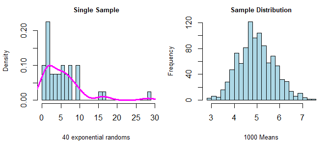
In the first graph, I show a single sample to illustrate the skew of an exponential distribution. The point is that the data are not normally distributed. The second graph shows the distribution of the means of 1000 simulated exponential samples, and the data appear normally distributed.

The theoretical distribution

The theoretical sample mean for an exponential distribution is 1/lambda. Lambda was given at 0.2, so the theoretical sample mean is 1/.2 = 5. Summarizing the data from our simulation of 1000 exponentials shows both the range and average of those means. The central limit theorem suggests that when n is large enough, the mean of the sample mean should approach the true mean. There appear cases when a single sample mean appears far from the theoretical mean (the min and max values below). Given our assumption of normality, however, we can assume that our sample’s mean will fall within two standard deviations of the true mean 95% of the time.

summary(Ksims)

##    Min. 1st Qu.  Median    Mean 3rd Qu.    Max. 
##   2.858   4.444   4.922   4.971   5.488   7.557

par(mfrow=c(1,1))
hist(Ksims, col="chartreuse", breaks=20, main="Sample Distribution with Mean",
     cex.main=.8, xlab="Means", ylab="frequency", cex.lab=.8)
abline(v=mean(Ksims), lwd=3, col="magenta")

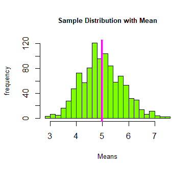
Indeed, the observed sample mean is approximately the theoretical mean; or, we may say that ‘the estimator is consistent.’ In the figure below, the pink verticle line represents the sample mean; we see that it is drawn approximately where x = 5.

How Vary Convenient

The LLN works for other statistics too. Given that the CLT suggests that the sample mean is normally distributed, and given that we found that the sample mean is a consistent estimate, we should expect that the variance of the sample mean is consistent as well. We can compare the theoretical variance to our sample variance.

The theoretical variance of a random exponential sample is (1/lambda)^2 = 25. The theoretical variance of the sample mean (standard error squared) is:

((1/lambda)/sqrt(n))^2

## [1] 0.625

Which we can compare to the variance of our simulation:

var(Ksims)

## [1] 0.6215836

We see that these are vary similar. Like with the theoretical and observed mean, the central limit theorem suggests that when n is large enough the observed variance should approach the true variance.

##

Finally, the central limit theorem states that as n increases, the sample mean is normally distributed. Below, I compare the density curve of our simulated means to a theoretical normal distribution.

hist(Ksims, prob=TRUE, col="chartreuse", breaks=20, 
     main="Sample Distribution with Density Curves", cex.main=.8,
     xlab="Means", ylab="Frequency", cex.lab=.8)
lines(density(Ksims), col="magenta", lwd=3, lty=1)

xfit<-seq(min(Ksims),max(Ksims),length=n^2)
yfit<-dnorm(xfit, mean=mean(Ksims),sd=sd(Ksims))
lines(xfit, yfit, col="black", lty=2, lwd=2)

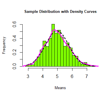
Our sample distribution appears approximately normal.

Conclusion

The LLN and CLT provide the basis for statistical inference. When n is large enough, we can use our statistical estimates to make informative comparisons. Because we can assume normality of sample means, we can use the properties of the normal distribution to examine the probability that two samples are meaningfully different. Importantly, this is true for population distributions that are non-normal in the first place.