Fantasy BBall Ranking Optimization for Category Leagues
In this project I use Principal Components Analysis to uncover the covariance structure of NBA stat production and apply it to fantasy basketball scoring categories through a system of Structured Hierarchically Adjusted Weights (SHAW). I evaluate my SHAW ranking metric against traditional Z-score rankings using top-n matchups and draft-simulated leagues, showing that SHAW rankings consistently and convincingly produce teams that win head-to-head matchups. The result is a game-theoretically informed ranking system optimized for how fantasy basketball actually determines winners.
Contents
- 00. Project Overview
- 01. Data Preprocessing
- 02. Traditional Z-scores
- 03. Covariance Matrix
- 04. Principal Components Analysis
- 05. SHAW Category Weighting
- 06. Ranking Comparisons
- 07. Conclusion
Project Overview
Fantasy basketball is a popular pastime with over 20 million participants in the U.S. and Canada anually (FSGA.org). In a fantasy basketball league, participants create a team by drafting from a pool of NBA players, whose real-game stats become their own fantasy stats for the season. Success requires knowing the players and understanding the league’s scoring format. In standard nine-category leagues, teams compete in weekly matchups across nine statistical categories (Points, 3-Pointers Made, Field-Goal %, Free-Throw %, Rebounds, Assists, Steals, Blocks, and Turnovers, which count against you). The matchup winner is the team that wins the most categories.
For example:
Table 1. Example Nine-Category League Matchup
| Team | Points | 3-pointers | Field-Goal % | Free-Throw % | Rebounds | Assists | Steals | Blocks | Turnovers | Total Categories | Matchup Winner |
|---|---|---|---|---|---|---|---|---|---|---|---|
| A | 600 | 75 | 48.7 | 83.5 | 239 | 72 | 43 | 30 | 90 | 4 | |
| B | 700 | 78 | 46.2 | 81.5 | 212 | 85 | 45 | 22 | 66 | 5 | X |
Although player histories and stat profiles are known, identifying the best draft choices is difficult when players are good in some categories but not others. To help managers choose, major platforms like Yahoo and ESPN include player rankings. These rankings are based on Z-scores: they standardize players’ statistics across scoring categories and then rank the sums. Z-score rankings are great at ordering players by total statistical output, but in a competitive league environment with rules and constraints (finite categories, position requirements, draft order, etc.), managers must make strategic decisions about which players are more useful to a specific team-build, not just better in the abstract.*
I propose a game-theoretical improvement on existing fantasy basketball rankings that works by leveraging the covariance structure of NBA stats using Principal Components Analysis. Rather than focusing on individual players who are strong in multiple categories (as Z-scores do), this method shifts the focus to the stat categories that covary the most within the player population.
For regular fantasy basketball managers, this idea is intuitive: NBA stats tend to bundle in a few player archetypes:
- Guards/Playmakers: assists, points, 3-pointers, FT%, turnovers
- Bigs: rebounds, blocks, FG%
- Wings/3 & D players: steals, 3-pointers
Because conventional nine-category leagues disproportionately reward the guard/playmaker cluster of categories (see above, 5 categories vs. 3), a clear implication follows: weighting categories based on this covariance structure identifies players who offer compound value, even if they are not the most productive across all statistical categories.
I map this covariance structure onto a league’s scoring categories using Structured Hierarchical Adjusted Weights (SHAW). I then build and evaluate ranking metrics using top-N-player matchups and simulated league/drafts, demonstrating that my covariance-tuned ranking method dramatically outperform traditional Z-score approaches in head-to-head matchups.
Actions
For a literature review and discussion of my previous attempts to improve fantasy rankings, see the ‘theory & discussion’ page in this project’s home repository:
The following is a simplified discussion and demonstration of:
- Standard Z-score approach, reproduced here for a baseline comparison metric
- Covariation Analysis to explore how fantasy categories relate to each other
- Principal Components Analysis to identify statistical structures
- SHAW category weighting to apply these structures to build a ranking metric
- Top-N evaluation comparing head-to-head category value across ranking systems
- Simulated draft evaluation assessing how ranking systems perform in draft-and-play scenarios
Results
My SHAW ranking system consistently outperforms traditional Z-score rankings in two tests using player per-game nba season data.
Top N Matchups
When comparing the top players in each ranking - at each of the top 150 levels (i.e., top 1 vs. 1, top 2 vs. top 2, … , top 150 vs. top 150) SHAW rankings win matchups 87 - 97 percent of head-to-head matchups over the last five NBA seasons. That indicates that at almost every depth, my metric consistently pulls matchup value towards the top of the rankings.
Draft-Simulated Leagues
In simulated league matchups (10-team snake drafts repeated ten times per season), one team drafts using SHAW rankings and the other nine teams draft using the standard Z-score rankings. This setup mirrors a realistic league environment where a single manager employs an optimized strategy while the rest follow conventional rankings. Across these simulations, SHAW-drafted teams win 64–100 percent of matchups against the nine standard-drafted opponents. SHAW teams also finish in the top 3 of the 10-team league 70–100 percent of the time.
Table 2. SHAW rankings vs. Traditional Z-score rankings
| Season | Top-N matchup win rate | Top-N category win rate | Simulated Draft - Matchup Win Rate | Simulated Draft - League Top 3 |
|---|---|---|---|---|
| 2020-21 | 96.7% | 55.1% | 93.3% | 100% |
| 2021-22 | 91.3% | 55.0% | 100% | 100% |
| 2022-23 | 94.7% | 55.0% | 66.7% | 70% |
| 2023-24 | 91.3% | 55.6% | 81.1% | 90% |
| 2024-25 | 87.7% | 54.9% | 64.4% | 70% |
| 2025-26 (Nov/26) | 91.6% | 55.1% | 87.8% | 100% |
Although these comparisons are based on static season averages, the results are strong and consistent. If nothing else, this shows that the top players in a Z-score ranking system can be rearranged to produce head-to-head matchup wins in a stable, repeatable fashion. This ranking system does come with a tradeoff. It does not produce teams that are balanced across categories. In fact, it consistenly wins by winning (the same) 5 of 9 categories. My metric thus implies a game-theoretical strategy: value the cluster of categories that wins matchups, but fantasy managers must stay flexible and savvy to identify best draft selections in real league scenarios.
Data Preparation and Preprocessing
NBA season data (including up to date current season stats) can be found using the nba_api package in Python. For more information see (https://github.com/swar/nba_api). Season data goes back many years, so users can change the season parameter to test this metric against past seasons.
from nba_api.stats import endpoints
from nba_api.stats.endpoints import LeagueDashPlayerStats

import os
import pandas as pd

# os.chdir("C:/Data Projects/NBA")
# To change the season, use this format: "YYYY-YY"
season = "2024-25"

def fetch_player_stats():
    player_stats = LeagueDashPlayerStats(season=season)
    df = player_stats.get_data_frames()[0]
    return df

nba_raw = fetch_player_stats()
Minimum Viable Player Pool
Z-scores measure one’s contributions relative to the average player, so it matters what subset of players are included in the fantasy population. Every season, there are about 500-600 players that will play in the NBA, but only about 300 will make consistent statistical impacts. If low usage players are included in the population, skewed NBA stat distributions become more extreme, which is not necessary since many of those players would not be rostered in a fantasy league. Common practice seems to be to include about 350 in the minimum viable player population.
I include players that average at least 15 minutes-per-game, and have played in at least 15% of a season’s games. A 15 minutes-per-game minimum corresponds roughly to a (minimum) permanent rotation player. Below that threshold, players introduce noisy variance that never affects a fantasy league because they are never rostered. These cutoffs typically results in a player pool of about ~350 players, whom average ~25 minutes per game.
# Preprocess/Subset viable players

# Define GP and MPG subset thresholds
min_games = nba_raw['GP'].quantile(0.15)
nba_raw['mpg'] = nba_raw['MIN'] / nba_raw['GP']

# Subset viable players
nba_subset = nba_raw[
    (nba_raw['GP'] >= min_games) &
    (nba_raw['mpg']>= 15)
].copy()
Thus, the relevant per-game data columns with player-names, games-played, and minutes-per-game included:
Table 3. 2024-25 per-game stats for a random sample of players
| Player | GP | mpg | FG_PCT | FT_PCT | FGA | FGM | FTA | FTM | FG3M | PTS | REB | AST | STL | BLK | TOV | |
|---|---|---|---|---|---|---|---|---|---|---|---|---|---|---|---|---|
| 310 | Jusuf Nurkić | 51 | 20.84 | 0.48 | 0.66 | 6.9 | 3.29 | 2.51 | 1.67 | 0.63 | 8.88 | 7.8 | 2.25 | 0.78 | 0.67 | 1.9 |
| 374 | Malcolm Brogdon | 24 | 23.5 | 0.43 | 0.88 | 10 | 4.33 | 3.83 | 3.38 | 0.67 | 12.71 | 3.79 | 4.08 | 0.54 | 0.21 | 1.58 |
| 222 | Jaime Jaquez Jr. | 66 | 20.73 | 0.46 | 0.75 | 7 | 3.23 | 2.15 | 1.62 | 0.56 | 8.64 | 4.39 | 2.52 | 0.92 | 0.21 | 1.48 |
| 340 | Klay Thompson | 72 | 27.29 | 0.41 | 0.9 | 12.18 | 5.01 | 1.03 | 0.93 | 3 | 13.96 | 3.42 | 2.01 | 0.69 | 0.42 | 1.22 |
| 562 | Zach Collins | 64 | 15.27 | 0.51 | 0.88 | 4.72 | 2.39 | 1.22 | 1.08 | 0.5 | 6.36 | 4.5 | 1.73 | 0.45 | 0.45 | 0.94 |
| 204 | Ivica Zubac | 80 | 32.8 | 0.63 | 0.66 | 11.78 | 7.4 | 2.95 | 1.95 | 0 | 16.75 | 12.62 | 2.68 | 0.69 | 1.12 | 1.59 |
Transformations
Percentage categories are scaled by player attempts. Take the player’s percentage difference from the mean (or, ‘deficit’) and multiply by their attempts. The result is a percentage ‘impact’ score that is then standardized.
Because turnovers count against a team, I reverse code them so that Z-scores can be simply added.
Thus, the scoring categories that will be standardized include:
Table 4. 2024-25 ‘fantasy-scoring’ per-game stats for a random sample of players
| Player | FT_impact | FG_impact | PTS | FG3M | REB | AST | STL | BLK | tov | |
|---|---|---|---|---|---|---|---|---|---|---|
| 322 | Kelly Olynyk | -0.04 | 0.2 | 8.73 | 0.75 | 4.68 | 2.91 | 0.75 | 0.43 | -1.73 |
| 426 | Noah Clowney | 0.09 | -0.88 | 9.13 | 1.89 | 3.93 | 0.87 | 0.52 | 0.46 | -1 |
| 490 | Shai Gilgeous-Alexander | 0.99 | 1.13 | 32.68 | 2.14 | 4.99 | 6.39 | 1.72 | 1.01 | -2.41 |
| 545 | Tyrese Maxey | 0.52 | -0.63 | 26.33 | 3.1 | 3.35 | 6.1 | 1.75 | 0.4 | -2.38 |
| 183 | Grant Williams | 0.12 | -0.22 | 10.38 | 1.69 | 5.12 | 2.31 | 1.12 | 0.81 | -1.75 |
| 478 | Russell Westbrook | -0.39 | -0.2 | 13.25 | 1.25 | 4.93 | 6.09 | 1.41 | 0.49 | -3.23 |
Traditional Z-scores
The standard method used by fantasy analysts, and implemented by major sites like Yahoo, ESPN, and Basketball Monster, is to:
- Standardize each category
- Sum the Z-scores across categories
- Rank players by the summed value
# Z score Function
def Z(stat):
    return (stat - stat.mean())/stat.std()
Because fantasy scoring categories exist on different scales (e.g., more points accumulate than rebounds, and more steals accumulate than blocks), we standardize to put the different categories on the same scale. Z-scores tell us how many standard deviations a player is from the mean in a category. So instead of comparing, say, 22 points-per-game vs. 10 rebounds-per-game, we can compare 2 standard deviations above the mean in any given category to 1.5, with clear implications, all other things being equal.
ESPN and Yahoo appear to adjust Z-score rankings by forecasting (perhaps given team dynamics like injuries which can change a players’ usage), but their formulas for doing so are opaque. In any case, their rankings do not fare well against the straightforward Z-score model when comparing players’ per-game stats.
Basketball Monster, a well-known fantasy baskeball analystics site also uses Z-scores as a baseline, and makes adjustments that purport to improve upon Z-scores alone. Their methods are also proprietary and hidden, but I’ll show later that there is little evidence that their adjustments make any improvement.
I reproduced Z-score rankings to serve as a baseline comparison here.
scoring_cats = ['FT_impact', 'FG_impact', 'PTS', 'FG3M', 'REB', 'AST', 'STL', 'BLK', 'tov']
z_df = pg_stats[scoring_cats].apply(Z)
Thus, per-game stats, standardized, added, and ranked.
Table 5. 2024-25 top 6 Z-ranked players & Giannis Antetokounmpo
| Player | FT_impact_z | FG_impact_z | PTS_z | FG3M_z | REB_z | AST_z | STL_z | BLK_z | tov_z | Z_sum | Z_rank | |
|---|---|---|---|---|---|---|---|---|---|---|---|---|
| 423 | Nikola Jokić | 0.377017 | 3.70272 | 2.83457 | 0.590496 | 3.47915 | 3.92079 | 2.57391 | 0.277659 | -2.23121 | 15.5251 | 1 |
| 490 | Shai Gilgeous-Alexander | 3.95662 | 1.9759 | 3.34211 | 0.780825 | 0.130278 | 1.88137 | 2.32634 | 1.12494 | -1.15249 | 14.3659 | 2 |
| 550 | Victor Wembanyama | 0.830546 | 0.293326 | 1.96236 | 1.81558 | 2.72662 | 0.422462 | 0.70527 | 7.5612 | -2.17397 | 14.1434 | 3 |
| 28 | Anthony Davis | -0.298244 | 1.52482 | 2.03846 | -0.820876 | 2.97214 | 0.367588 | 0.777485 | 3.74185 | -0.916293 | 9.38693 | 4 |
| 543 | Tyrese Haliburton | 0.796741 | 0.145011 | 1.03779 | 1.70504 | -0.49692 | 3.38384 | 1.54667 | 0.342585 | -0.213567 | 8.24719 | 5 |
| 314 | Karl-Anthony Towns | 0.989625 | 1.7362 | 1.99015 | 0.591367 | 3.49423 | 0.119866 | 0.310903 | 0.395696 | -1.47049 | 8.15754 | 6 |
| 180 | Giannis Antetokounmpo | -7.08645 | 4.59862 | 2.966 | -1.34507 | 3.11973 | 1.91752 | -0.0182002 | 1.47049 | -1.97181 | 3.65082 | 58 |
These values illustrate how total Z-score rankings emerge from category-level contributions and help motivate the critique discussed below. A seasoned fantasy manager may notice here that the top 6 Z-ranked players represent different player types:
** Jokic and SGA: both multi-category superstars, one a ‘point center’, another a perimeter playmaker. ** Wemby: An extreme outlier in one scarce category. ** AD: Interior ‘big’ ** Haliburton: High assist ‘gaurd/playmaker’ ** KAT: Stretch ‘big’
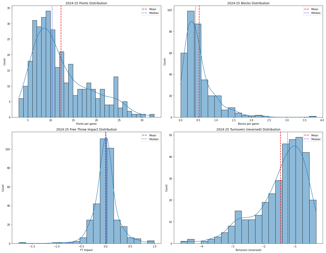
Distributions & Critique
A common critique of Z-score rankings is that because NBA stat distributions are skewed, standardized scores “distort” a player’s value. (A mistaken version of this claims we should not standardize at all when distributions are non-normal) The critique is compelling at first glance, but I argue that it is slightly misguided.
To the misguided critique: Z-scores do not assume normal distributions because they are not being used for statistical tests; they only measure standardized distance from the mean. Skew affects interpretation but not validity.
Two examples illustrate the more compelling concern:
** Victor Wembanyama shows extreme positive skew in Blocks. In the table above, more than half of his total Z-score comes from a single category. Critics may worry that his value is “too concentrated,” as fantasy outcomes depend on winning multiple categories, not just one.
** Giannis Antetokounmpo, by contrast, appears to be underrated. His −7 FT_impact score drags his Z_sum down to 3.6, dropping him from a hypothetical #4 (if he were league-average at free throws) to #58. Critics may argue that this hides the fact that he contributes strongly across many other categories, and again, fantasy outcomes depend on winning many categories.
At a glance, these seem like two different problems, one of overstated value (Wemby), and one of understated value (Giannis). But they are actually opposite sides of the same concern: that skewed NBA distributions imply a flaw in how Z-scores represent value.
But the math is correct. Wemby really does help you in Blocks and Giannis really does hurt you in Free throws. The real issue is not skew; it is not how Z-scores are calculated; it is how Z-scores are aggregated. Summing across categories implicitly assumes that each category contributes independently to fantasy success. But fantasy matchups are not won by maximizing total value — they are won by winning five out of nine categories. Managers that think strategically should be concerned with combinations of categories, not about their summed magnitudes.
This is why the critique feels intuitively right: analysts know that multi-category performance matters, but the Z_sum formula treats categories as interchangeable and independent.
To be clear, Z-scores themselves are not the problem. Standardization is appropriate: player value should be understood relative to the league average in each category. Wemby’s extreme Blocks production is strategically valuable because scarcity matters. Giannis’s FT weakness is strategically costly because it directly affects one of nine winnable categories.
The real limitation of Z-score rankings is therefore not the standardization, but the assumption of independence baked into the summation step. To examine how fantasy categories actually relate to one another, we turn to the covariance matrix and Principal Components Analysis (PCA).
Covariance Matrix
If the core issue is that categories are treated as independent when they may not be, then the natural next step is to examine how they actually relate to one another in practice. Do certain categories tend to move together? Do some move in opposite directions? Do players naturally fall into multi-category “bundles” that Z-scores overlook?
To explore this, I isolated the nine standard fantasy scoring categories and computed a Pearson correlation matrix. To see whether Z-scores overlook meaningful relationships between categories, we first examine how the nine scoring categories co-vary.
scoring_cats = ['FT_impact', 'FG_impact', 'PTS', 'FG3M',
                'REB', 'AST', 'STL', 'BLK', 'TOV']

# Category correlation matrix
R = pg_stats[scoring_cats].corr().round(3)
Correlation coefficients tell us how strongly two numeric variables are associated, or how they vary together. A coefficient of 1 would indicate a perfect alignment (a 1-unit increase in x comes with a 1-unit increase in y).
Table 6. Covariance Matrix
| FT_impact | FG_impact | PTS | FG3M | REB | AST | STL | BLK | tov | |
|---|---|---|---|---|---|---|---|---|---|
| FT_impact | 1 | -0.388 | 0.322 | 0.552 | -0.288 | 0.302 | 0.106 | -0.258 | -0.221 |
| FG_impact | -0.388 | 1 | 0.141 | -0.451 | 0.625 | -0.06 | -0.012 | 0.454 | 0.009 |
| PTS | 0.322 | 0.141 | 1 | 0.605 | 0.403 | 0.676 | 0.415 | 0.153 | -0.798 |
| FG3M | 0.552 | -0.451 | 0.605 | 1 | -0.209 | 0.403 | 0.255 | -0.23 | -0.403 |
| REB | -0.288 | 0.625 | 0.403 | -0.209 | 1 | 0.173 | 0.148 | 0.625 | -0.373 |
| AST | 0.302 | -0.06 | 0.676 | 0.403 | 0.173 | 1 | 0.509 | -0.069 | -0.826 |
| STL | 0.106 | -0.012 | 0.415 | 0.255 | 0.148 | 0.509 | 1 | 0.074 | -0.447 |
| BLK | -0.258 | 0.454 | 0.153 | -0.23 | 0.625 | -0.069 | 0.074 | 1 | -0.126 |
| tov | -0.221 | 0.009 | -0.798 | -0.403 | -0.373 | -0.826 | -0.447 | -0.126 | 1 |
There are many strong correlations here, notably:
Turnovers are strongly associated with both points and assists. This makes intuitive sense: players that handle the ball a lot (i.e., are responsible for making plays by passing or scoring) end up losing it more often.
Rebounds are positively associated with Field Goal impact and Blocks. This also makes a lot of sense: Players that play closer to the basket (‘bigs’) get rebounds, blocks, and closer shots which brings up their field goal percentage.
Correlations only tell us about pairs of categories at a time, they do not reveal a broader structure. To get a picture of how all nine categories vary at once, we turn to Principal Components Analysis.
Principal Components Analysis
PCA is used to reduce a large set of correlated variables into a smaller number of dimensions or “components” that still capture most of the information in the data. Instead of looking at nine categories one pair at a time, PCA can reveal the underlying “stat ecosystem” that structure fantasy basketball production.
Conceptually: If several categories consistently rise and fall in tandem (like rebounds, blocks, and FG impact), PCA treats them as a single statistical “direction.” If other categories consistently oppose them (like points, assists, and FT impact), PCA identifies that tension as a separate dimension. PCA does not rank players; t shows how the categories related to each other, and that is what is missing from summed Z-scores.
Because fantasy categories exist on very different scales, PCA is performed on the correlation matrix (equivalent to PCA on standardized variables), ensuring equal weighting across categories.
pca_vars = PCA()
pca_vars.fit(R.values)
The PCA algorithm will produce:
- A PC (or’component’) for each of the nine variables
- A loading score showing how strongly each variable relates to that component
- And an “explained variance” ratio.
- An eigenvalue can also be obtained for each PC (>1 indicates a meaningful component).
I focus on the first two components here, as together they explain over 90% of the total variance in the data.
Table 7. PCA Output for Two Components
| Category | PC1 | PC2 |
|---|---|---|
| FT_impact | -0.336 | 0.275 |
| FG_impact | 0.268 | -0.412 |
| PTS | -0.389 | -0.289 |
| FG3M | -0.434 | 0.168 |
| REB | 0.092 | -0.535 |
| AST | -0.436 | -0.224 |
| STL | -0.263 | -0.17 |
| BLK | 0.188 | -0.396 |
| tov | 0.417 | 0.347 |
| Variance Explained | 0.573 | 0.341 |
| Eigenvalue | 1.194 | 0.71 |
The sign of a loading does not reflect whether a stat is “good” or “bad” for for the PC, only how that stat covaries with the others. Because turnovers are reverse-coded (higher values hurt you), they naturally load in the opposite direction of positively rewarded production stats.
PC1 (~57% of variance) primarily separates the nine categories into two coherent statistical bundles:
Interior / Efficiency Cluster (3 categories)
- Field Goal Impact
- Rebounds
- Blocks
Perimeter / Usage Cluster (6 categories)
- Free-Throw Impact
- Points
- 3-Pointers Made
- Assists
- Steals
- Turnovers (because it is reverse-coded we can interpret its negative sign as reflecting penalty scoring, while still varying with this cluster)
This component captures the strongest pattern of shared movement across fantasy statistics.
PC2 (~34% of variance) reveals a second, independent contrast that again separates interior actions (REB, BLK, FG impact) from perimeter creation (PTS, AST, FG3M, FT impact, and TOV). Although distinct from PC1, it reinforces the same underlying structure.
PCA does not impose positions or roles, but the statistical structure implies:
Fantasy production naturally organizes into a six-category perimeter cluster and a three-category interior cluster. This 6–3 pattern describes how categories actually move together in NBA data. The reverse coding of turnovers merely flips their direction, not their group membership.
This structure becomes the foundation for rethinking player value beyond simple additive Z-scores—because it suggests that categories are not independent silos, but parts of two larger statistical ecosystems.
To make the PCA structure more interpretable, I visualize the first two principal components with a PCA biplot, and the pairwise relationships among categories with a hierarchical clustering dendrogram.
# PCA Biplot

pca = PCA(n_components=2)
pca.fit(R.values)
loadings = pca.components_.T

plt.figure(figsize=(6, 6))
...
plt.show()

# Dendogram

cm = sns.clustermap(
    R,
....
plt.show()
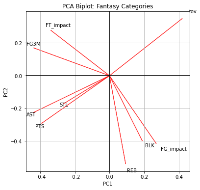
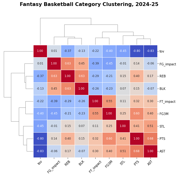
The biplot projects each category into the PC1–PC2 space. Categories that point in similar directions (and lie near each other) tend to move together; categories that point in opposite directions tend to trade off. The dendrogram then reclusters the correlation matrix, grouping categories into tight clusters based on their similarity.
Taken together, the PCA and clustering visuals reinforce the idea that fantasy categories do not behave as nine independent dimensions. Instead, they fall into two coherent covariance bundles—a six-category perimeter cluster and a three-category interior cluster—which motivates reweighting categories in a way that respects this structure.
SHAW category weighting
The PCA and covariance analysis do not tell us how to rank players. But they do tell us that the nine fantasy categories are not equally independent. They organize into a 6–3 covariance structure:
- Six perimeter/usage guard/playmaker categories (PTS, FG3M, AST, STL, FT_impact, and turnovers) move together.
- Three interior/efficiency bigs categories (REB, BLK, FG_impact) move together.
Because turnovers belong to the belong to the perimeter cluster, but count as a penalty, the balance is:
- Guards/playmakers: 5 categories
- Bigs: 4 categories
A ranking system that treats all nine categories as equally independent is therefore ignoring real structure in how basketball production actually co-varies. This means, on average, a player tends to belong to one of these statistical clusters. When a high usage perimeter player is drafted, the manager is likely getting value across five categories. When an interior ‘big’ is drafted, the manager is likely getting value across four categories. Now, because these categories primarily move in different directions - that is the ‘guard’ players are likely low in the ‘big’ categories, and vice versa, drafting one of each may give a team balance, but may actually reduce overall matchup efficacy. Now, it should be evident that: to tilt a team-build towards ‘bigs’ is to maximize four of nine categories, but to tilt a team towards guards/playmakers is to maximize in five of nine categories. Tilting toward perimeter production maximizes access to more winnable categories.
SHAW (Structured Hierarchical Adjusted Weights) is my attempt to incorporate this structure without abandoning the basic logic of standardized scores.
The SHAW approach does two things:
- It up-weights the dominant (perimeter/usage) cluster
- It down-weights the subordinate (interior/efficiency) cluster
This creates a hierarchy that reflects the covariance structure revealed by PCA: perimeter creation drives the most variation in fantasy production, but interior efficiency still matters.
The weights themselves were derived through a combination of PCA-informed structure and a controlled guess-and-check performance test. I iteratively adjusted weights in increments of 0.1 or 0.05 and compared the resulting rankings against Traditional Z-scores using Top-N matchup simulations (see results below). The weights that produced the best overall results are:
# Define Weights
shaw_weights = {
    'PTS':       1.15,
    'FG3M':      1.25,
    'REB':       0.60,
    'AST':       1.00,
    'STL':       1.25,
    'BLK':       0.60,
    'FT_impact': 1.00,
    'FG_impact': 1.00,
    'tov':       0.85,
}

shaw_z = Z(pg_stats[scoring_cats])

for cat in scoring_cats:
    shaw_z[cat] = shaw_z[cat] * shaw_weights[cat]
Assists, and percentage categories were left unchanged. That is because, given the other weights, changing these did not make much difference in the outcome.
Next, rather than simply adding those weighted Z-scores, I include a clip of the lower tail. Z-scores lower than -3.8 are clipped. This practice only affects distributions that have a negative skew, which is only turnovers (because they are reverse coded) and Free-throw impact (which can have a long negative tail because bad shooters can have lots of attempts).
pg_stats[ [f"{c}_shaw_z" for c in scoring_cats] ] = shaw_z

# Clipped Z scores
def clippedZ(stat, lower=-3.8, upper=None):
    return stat.clip(lower=lower, upper=upper)
With weighted and clipped Z-scores, SHAW rankings can now be compared directly against traditional Z-scores in matchup simulations.
Ranking Comparisons
I compare my ranking system to the traditional Z-rankings as well as Basketball Monster (BBM) rankings.
I show the top 20 SHAW rankings, with the Traditional-Z BBM player ranks alongside them for comparison. BBM rankings track with Traditional Z-scores for the most part, but SHAW rankings begin to differ dramatically after n=15.
Table 8. 2024-25 SHAW vs. Traditional Z and BBM Rankings Table
| Player | SHAW_rank | Traditional_Z_rank | BBM_rank | |
|---|---|---|---|---|
| 266 | nikola jokic | 1 | 1 | 1 |
| 306 | shai gilgeousalexander | 2 | 2 | 2 |
| 336 | victor wembanyama | 3 | 3 | 3 |
| 70 | damian lillard | 4 | 7 | 8 |
| 331 | tyrese haliburton | 5 | 5 | 5 |
| 233 | luka doncic | 6 | 8 | 7 |
| 309 | stephen curry | 7 | 9 | 9 |
| 333 | tyrese maxey | 8 | 11 | 10 |
| 223 | kyrie irving | 9 | 12 | 12 |
| 149 | james harden | 10 | 14 | 15 |
| 209 | kevin durant | 11 | 10 | 11 |
| 21 | anthony edwards | 12 | 15 | 16 |
| 163 | jayson tatum | 13 | 13 | 13 |
| 102 | dyson daniels | 14 | 18 | 14 |
| 194 | karlanthony towns | 15 | 6 | 6 |
| 147 | jamal murray | 16 | 16 | 18 |
| 20 | anthony davis | 17 | 4 | 4 |
| 91 | devin booker | 18 | 28 | 33 |
| 322 | trae young | 19 | 44 | 51 |
| 229 | lebron james | 20 | 17 | 20 |
The top three valuable players in each of the rankings is the same. These players are so elite that changing the calculus does not impact their position. Anthony Davis on the other hand, drops from #4 to number #17 in my ranking. He is elite in rebounds and blocks, two categories that are weighted down in my system. Note that Nikola Jokic and Victor Wembanyama are both ‘bigs’. Jokic gets a lot of rebounds and Wembanyama gets a lot of blocks. But they are also good enough in enough other categories to remain at the top of the ranks. That is, although they are ‘bigs’, they still score in the dominant cluster of categories. In the remaining top 20, we see the down shift of other bigs that are elite in rebounds (KAT) and a shift up from playmakers (Lillard, Doncic, Harden), sometimes dramatically (Trae Young). A lot of players might remain in the same positions but for different reasons (e.g., Durant, Murray).
My ranking does not suppose that Anthony Davis is now only the 17th best player. Rather, my rankings suppose that, given the scoring categories that matter for matchups in Fantasy basketball, Anthony Davis’s statistical output does not ‘fit’ as well as Damian Lillard’s.
Top-N comparisons
To evaluate this formally, I run a controlled head-to-head simulation.
For each n from 1 to 150, I:
- Select the top n players from each metric.
- Aggregate their per-game stats to form a hypothetical “Top-n Team.”
- Compare those teams across all nine categories.
- Record:
- Category wins (out of 9)
- Matchup wins (win = 1, tie = 0.5)
This produces:
- 150 matchups per season per comparison
- 1350 category-level comparisons per season
Top-N teams test whether a ranking method places the right players at the top, because in real drafts, early selections determine the rest of the team’s structure. Matchup wins are especially meaningful because fantasy weeks are decided by matchups, not total accumulated value.
# full implementation available in the repo
def generate_summary_dfs(...):
    ...

def compare_summary_dfs(...):
    ...
For every season and every ranking comparison, a cumulative head-to-head matchup summary shows how the rankings fare against each other. For example:
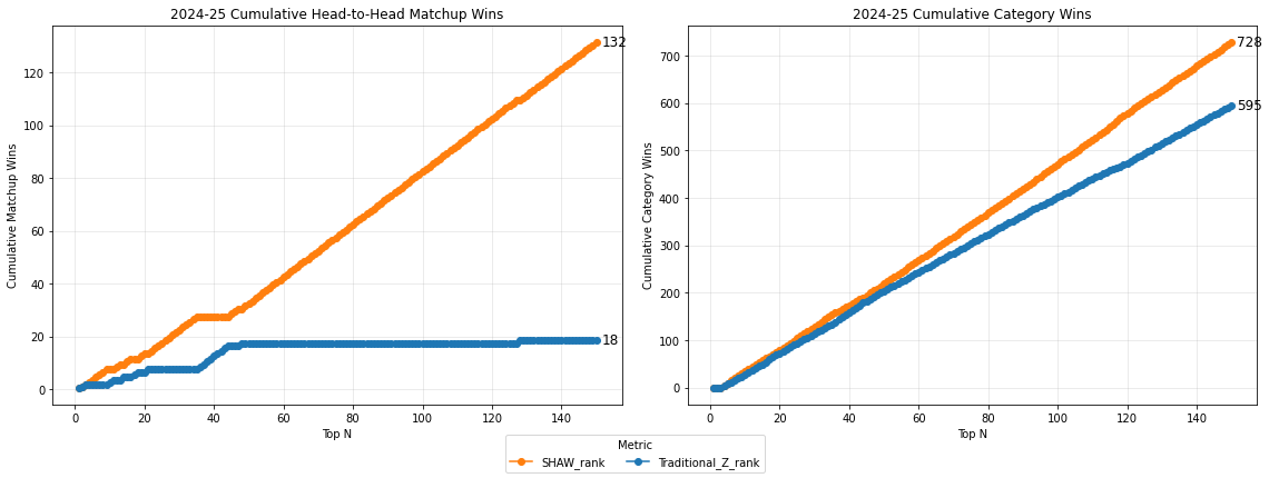
In the 2024-25 season, my SHAW ranking outperforms the Traditional Z-ranking by 132 matchup wins to 18, and 728 category wins to 595.
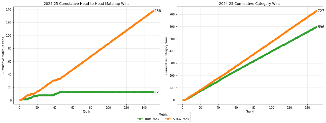
Against BBM rankings, SHAW rankings outperform by similar margins.
Shaw rankings dominate traditional Z rankings and BBM rankings by large margins in total matchup wins. This is true for every NBA season from 20-21 to 24-25.
Table 9. Top-N matchup and Category wins vs. Traditional & BBM rankings
| Season | Shaw vs Trad (Matchups) | Shaw vs Trad (%) | Shaw vs Trad (Cats) | Shaw vs Trad Cat (%) | Shaw vs BBM (Matchups) | Shaw vs BBM (%) | Shaw vs BBM (Cats) | Shaw vs BBM Cat (%) |
|---|---|---|---|---|---|---|---|---|
| 2020-21 | 141-9 | 94.0 | 732-597 | 55.1 | 133-13 | 88.7 | 721-607 | 54.3 |
| 2021-22 | 140-10 | 93.3 | 741-585 | 55.9 | 134-16 | 89.3 | 730-596 | 55.1 |
| 2022-23 | 141-9 | 94.0 | 743-607 | 55.0 | 143-7 | 95.3 | 745-605 | 55.2 |
| 2023-24 | 136-14 | 90.7 | 743-598 | 55.4 | 140-10 | 93.3 | 743-596 | 55.5 |
| 2024-25 | 132-18 | 87.7 | 728-595 | 55.0 | 138-12 | 92.0 | 727-596 | 55.0 |
Although SHAW rankings do not dramatically increase total category wins, it substantially increases matchup wins by concentrating value into category combinations that consistently beat opponents. In other words, SHAW wins efficiently, dominating the matchup wins even when total category margins are moderate. Traditional Z-scores distribute value across categories that do not reinforce each other, which leads to strong Z totals but weaker matchup performance. SHAW explicitly exploits covariance structure to avoid this inefficiency.
Simulated Draft Comparisons
Top-N comparisons are meaningful, but can react to small fluctuations in player position.
To further stress-test ranking behavior, I simulate 10 full snake drafts:
In each draft, one SHAW-drafted team competes against nine baseline-drafted teams, which sets a high bar: outperforming the field is far more demanding than outperforming a single metric.
- A 10-team league
- One team drafted using the “test” metric
- Nine teams drafted using the baseline metric
- The test team occupies draft positions 1–10 across simulations
- All resulting teams are compared across the nine categories
Table 10.
| Season | Matchup Win Rate | League Top 3 |
|---|---|---|
| 2020-21 | 93.3% | 100% |
| 2021-22 | 100% | 100% |
| 2022-23 | 66.7% | 70% |
| 2023-24 | 81.1% | 90% |
| 2024-25 | 64.4% | 70% |
| 2025-26 (Nov/26) | 87.8% | 100% |
All things being equal, SHAW rankings would expect to win matchups 50% of the time, and appear in the league-Top-3 30% of the time. Across all seasons and draft slots, however, SHAW-drafted teams consistently outperform baseline rankings, typically finishing among the top few teams in aggregate category strength and simulated matchup wins. These draft simulations demonstrate that the covariance-aware weighting is not only mathematically coherent—it produces strategically superior fantasy teams under realistic drafting constraints.
SHAW vs. Punt Strategies
Thus far I have suggested that my metric is a ‘game-theoretical’ improvement because it eschews overall player strength to exploit the payoff structure of the 9-category format, which is that you only need to win 5 of 9 categories to win a matchup. But I am not the first to ‘game’ the fantasy rules.
Punting is a well-known fantasy strategy in which a manager gives up on one or more categories with the hopes of concentrating value in several others. This might happen spontaneously in draft scenarios, as a manager takes stock of their team build and makes decisions on the fly about what category strengths to focus on and which to ‘give up.’ Or, managers might pursue a punt strategy from the beggining, perhaps anticipating certain category strengths give their assigned draft order.
I argue, however, that punting is a sub-optimal gaming strategy, even when it alligns with the covariance structure discussed above. Punting may beat Traditional Z-score rankings for select categores, but no punt builds beat SHAW rankings.
Turnovers looks like an obvious candidate if one wants to punt. Because high turnover players tend to be high in several other categories, in fact, it might even seem like high turnovers are a signal for compound value. In fact, one well known fantasy basketball ranking metric, Hashtag Basketball, is known to construct their Z-score based ranking simply by weighting turnovers by 0.25.
Let us see what happens if we ‘punt’ turnovers, or construct a Z-ranking that omits turnovers completely from the sum of Z-scores.
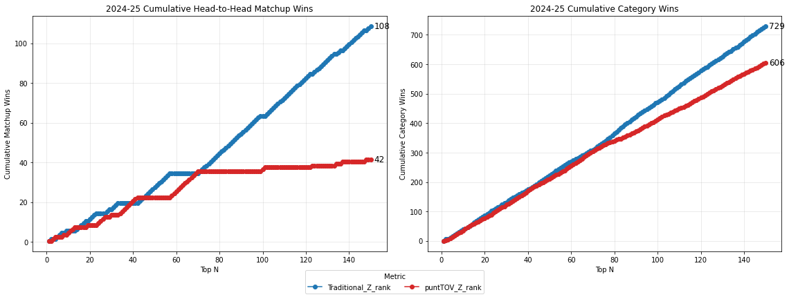
Against the standard (9-cat) Z-score ranking, the punt ranking does not fare well in Top-N matchups. It appears to do equally as well up to about n=70, and then tails off. It does better in the simulated draft scenario, but not convincingly, winning only 52% of the time.
I constructed punt (8-cat) rankings for each of the nine categories (omitted), and found that only two of them fare better than full 9-category Z-score rankings. Not surprisingly, these are rebounds, and blocks, two ‘big man’ stats, that covary with the minority cluster. Punting both rebounds AND blocks in the same metric, also wins in Top-N matchups, but completely colapses in simulated draft leagues.
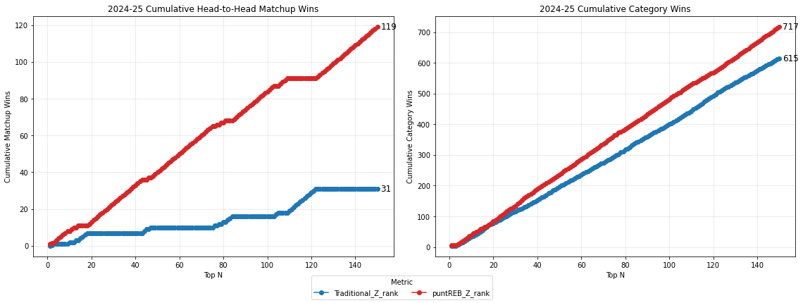
The punt-rebound ranking even places in the top 3 in 90% of simulated draft leagues (although punting blocks does no better than average). Punting rebounds is the only category that seems to optimize rankings for matchup wins in both Top-N matchups, and simulated drafts because removing it alone does not interfere with the covariance structure of the dominant cluster.
That said, a better way to treat rebounds (and blocks, and turnovers) is not to remove them, but to weight them down, as I have done in my SHAW ranking system. As such, my metric should beat a punt team by winning the categories punted, in addtion the categories up-weighted. Or, the trade-off for losing some upweighted categories some of the time would be off-set by winning the punted categories most of the time.
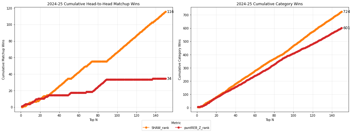
In simulated draft leagues, SHAW rankings beat punt-rebound ranked teams 77% of the time, and finished in the league top-3 80% of the time.
Conclusion
I developed a Structured Hieararchically Adjusted Weights (SHAW) ranking metric, based on the covariance structure of NBA stats production, and demonstrated clear improvements against Traditional Z-score rankings in nine-category head-to-head matchup leagues. Of the nine categories at stake in standard fantasy leagues, I find that six of them covary together, and in a different direction than the other three. Even though turnovers are a penalty, the balance (five to four) still favors one cluster over the other. To focus on the dominant cluster is to maximize compound value where it counts for fantasy scoring.
Critical observers might note that my method only ranks players for teams that win particular categories and not others, that I’ve created a system that appears to “punt” 4 categories in favor of 5. As such, I haven’t improved player rankings, I’ve just “hacked” the game.
The tests are reproducible
While I have used static, per-game season averages here to test my metric against the standard, the margins of improvement in Top-N comparisons and the consistent success in simulated drafts points to real findings.
The method is mathematically grounded
Weights are derived from the PCA-discovered covariance structure:
- A 6-category dominant cluster
- A 3-category subordinate cluster
SHAW is not punting
Punting removes a category from the calculus. SHAW includes all nine, even the categories it down-weights. In further analysis, I found that punting only works for select categories. And then, SHAW beats that same punt models by the same dramatic margins, because SHAW now wins in those minority categories too. Thus, my model should beat a ‘punt’ model all of the time.
Fantasy value is not real-basketball value
Traditional Z-score methods implicitly assume fantasy categories measure performance neutrally. But fantasy is a game, not unlike a market, with uneven payoff rules. The objective is not to estimate “true player performance.” It is to maximize expected wins under those rules. Like quantitative finance or the Moneyball model in baseball, the SHAW metric identifies and weighs sources of value that are mispriced by the current fantasy market. In this sense, fantasy basketball resembles quantitative trading more than player scouting: the winning strategy exploits structural inefficiencies in the scoring system.
A nine-category league does not reward ‘the best player’; it rewards players whose statistical portfolios align with the payoff structure of those nine rules. If that payoff structure disproportionately tracks the statistical profiles of one player archetype, then ranking systems that treat all categories as independent or equally valuable systematically ignores the optimal strategy. SHAW works because it models fantasy basketball as the covariation puzzle that it actually is, allocating value toward category combinations that maximize wins under the game’s payoff rules.
Application for K-category leagues
Nine-category leauges represent the standard, or default option. ESPN and Yahoo allow league commissioners to customize settings, however, with many more statistical categories (Double-Doubles, Triple-Doubles, 3-PT%, Assist-to-turnover ratio, etc.) available to add complexity and fun. For custom league categories, my method can be applied in the same way: A. use PCA to uncover the covariance structure of all the categories, and B. weight up to the dominant statistical cluster, and down the subordinate. For scenarios in which statistical clusters are relatively balanced, users should experiment with team-builds that move in either direction, or experiement with overlapping categories.
User Beware
Although my rankings beat the competition in head-to-head matchups, that does not mean that they would produce winning teams in real draft situations. They might, if other league members blindly subscribe to standard Z-rankings. 1. League rules still require managers to maintain players at each position, so any global ranking system alone will still require stategic choice about when to take a center vs. a gaurd, for example. 2. SHAW rankings represent a ‘game-theoretical’ improvement against a metric that does not know the scoring rules. Should every manager in a league adopt the same strategy implied by my ranking system, chances would be equal. If that is the case, ‘gaming the game’ would require adapting again, perhaps by adopting a strategy that focusses on the minority statistical cluster. 3. Finally, experienced managers should also know that draft day is only one variable in a fantasy season, as injuries, trades, and other events can change player output in ways that past per-game averages cannot predict. In conclusion, my rankings represent a strategic orientation towards optimal matchup performance, not a system that automatically wins.