Toy Robot: Toy Classification Using CNN
For this project I trained a Convolutional Neural Network to recognize distinct classes of toys from a bespoke, self-collected data set. After experimenting with various training parameters and model architectures, however, I used transfer learning - and the power of MobilenetV2 - to achieve a 100 percent test set accuracy. I conclude that CNN is all about optimizing model architecture and training parameters for the task, but building a successful model has much to do with the nature and quality of the data too.
Table of contents
- 00. Project Overview
- 01. Data Overview
- 02. Data Pipeline
- 03. CNN Overview
- 04. Baseline Network
- 05. Tackling Overfitting With Dropout
- 06. Image Augmentation
- 07. Learning Rate Reduction
- 08. Network Architecture
- 09. Transfer Learning
- 10. Overall Results Discussion
- 11. Next Steps & Growth
Project Overview
Context
I want to build a robot that will pick up my kid’s toys, AND put them in the correct bins! My four-year old - Teddy - is better at playing with toys than picking them up. I’m better at throwing them all in one basket than sorting them. I’m not a robotics engineer, but I can use Deep Learning techniques to train a computer to recognize a Brio from a Bananagram (among other toys), and I’ll leave the rest to my friends in the robotics lab.
I’ll use my own images of my kid’s toys as a unique, albeit limited, custom dataset, which will allow me to simulate the real world scenarios of toys scattered throughout the house.
If this is successful and put into place on a larger scale, no parent will ever step on a Lego again!
Actions
Thanks to the Keras Deep Learning library, most of the tasks and procedures for building a computer vision neural network are made easy in Python. On the other hand, while Keras provides the tools, understanding and optimizing the model’s architecture and training parameters is not so simple. Since I will be taking my own pictures, I also have to think hard about what constitutes good, useful data. The process of building this model, broken into subsections below, is as follows:
Generate Data:
- Take images.
- Structure the data into training, validation, and test set folders.
- Define the data flow parameters and set up data generator objects.
Iterative Model Building Method:
- I Start with a simple baseline model. The first network consists of: Two convolutional layers, each with 32 filters and subsequent Max Pooling Layers, A single Dense (fully connected) layer following flattening with 32 neurons, followed by an output layer for five toy classes, I use the RELU activation function on all layers, and I use the ‘ADAM’ learning optimizer
- Add a Dropout layer to reduce overfitting (which will be adjusted throughout)
- Add Image Augmentation to the data pipeline to increase variation in the training data, as well as address overfitting
- Add a Learning Rate Reducer to smooth convergence
-
Experiment with Layers and Filters: a. First adding more convolutional layer b. Increasing the filters in convolutional layers c. Decreasing the filters in the convolutional layers d. Increasing the kernel size
- Finally, I compare my network’s results against a Transfer Learning model based on MobilenetV2, a powerful CNN model that uses some advanced layering techniques.
Results
The baseline network suffered badly from overfitting, but the addition of dropout & image augmentation reduced this entirely (and led to underfitting). The addition of these learning parameters, however, only led to slight gains in model performance. Adding convolutional layers and filters also led to slightly better results. Switching to transfer learning made a huge difference, leading to 100% classification accuracy on the test set.
Classification Accuracy on the Test Set:
- Baseline Network: 74.7%
- Baseline + Dropout: 80%
- Baseline + Image Augmentation: 77.3%
- Baseline + Dropout + Image Augmentation + Learning Rate Reducer: 76%
- Architecture Experiment 2: 75.7%
- Architecture Experiment 4: 80%
- MobilenetV2 base model: 100%
The use of Transfer Learning with the MobilenetV2 base architecture was a bittersweet success. I wanted a more accurate model of my own, but it is hard to argue with the efficiency and predictive power of a network that will predict my kid’s toys 100% of the time. My small data set (500 training images) is less than ideal, but I’ve also learned to think very carefully about training data in CNNs.
Growth/Next Steps
The concept here is demonstrated, if not proven. I’ve shown that I can get very accurate predictions - that should this robot come to market, it will at least be able to accurately predict in what bins a childs’ toys belong.
I hold out that there is considerable room for improvement in my own, self-built model. The experimental architectures that I tested here does not exhaust the possibilities. I can use the Keras_tuner function to get an optimal network architecture. And/or, I can revisit my dataset, which is currently ‘small’ and is likely riddled with bias.
My current working hypothesis is that: with such limited data (100 images in each of my 5 training classes), the model is both sensitive to bias and lacks depth required to help a robot distiguish certain toys. I’ll explore this bias in the write up below. For now, I’ll note that the other image datasets that I’ve seen are either extraordinarily deep and diverse (Imagenet contains over 14 million images), or if they are smaller, appear to be produced in laboratory like conditions, with carefully controlled lighting and background. Although I was systematic in collecting the data for this project, my house (and my iphone camera) are far from laboratory conditions.
Data Overview
Although my kid has dozens of types of toys, I began with a modest set of five classes of toys:
- Bananagrams (a game for adults, which has become material for Teddy’s garbage truck)
- Brios
- Cars
- Duplos (big legos for younger builders)
- Magnatiles
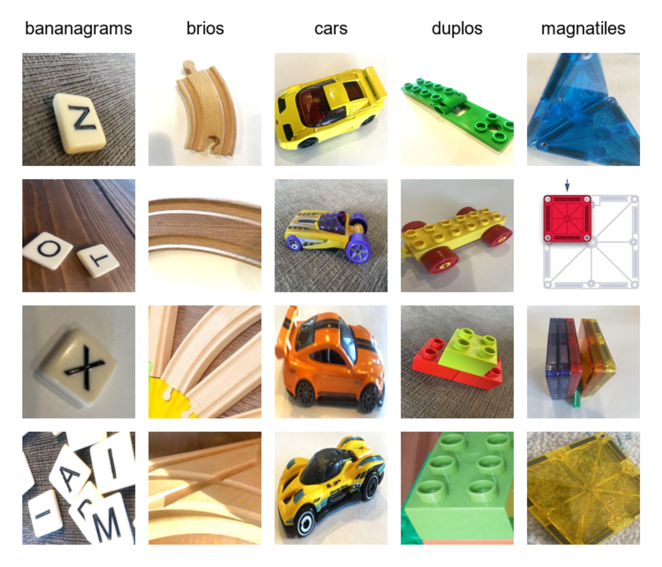
Problems: At first glance, these toys appear distinct enough, but when considering how an algorithm might think about them, some challenges arise. Duplos are mostly made of building blocks, but there are plenty of figurines, animals, and other structures that belong in the same toy bin. Duplos have distinct circular connectors, but they are also square-shaped, like bananagrams and magnatiles, and they are made of solid colors, like magnatiles and Brio cars. Brios, likewise, come with both natural-colored wooden train tracks and multi-colored train cars, which have wheels, like cars. Cars and Bananagrams are relatively small, which makes capturing images of the same proportions as the other toys quite difficult. While Teddy does have hundreds of Duplos and Brios to photograph, there are limited numbers of cars and magnatiles, which means my training, validation, and test sets will have multiple (however different) images of the same objects.
Solutions: To simplify, I removed the Duplo figurines and the Brio train cars from the sample population. After some trial and error, I also diversified and stratified the backgrounds for images in each toy class. Finally, I cropped most images so that the toy occupies the majority of the image frame. Because of the limited number of some types of toys, I separated the actual toys for the training, validation, and test set images.
I ended up with 145 images of each toy, separated as follows:
- 100 training set images (500 total)
- 30 validation set images (150 total)
- 15 test set images (75 total)
For ease of use in Keras, my data folder structure first splits the image data into training, validation, and test directories, and within each of those is split again into directories based upon the five toy classes.
Images in the folders are varying sizes, but will be fed into the data pipeline as 128 x 128 pixel images.
Data Pipeline
Before building the network architecture and then training and testing it - I use Keras’ Image Data Generator to set up a pipeline for the data to flow from my local hard-drive through the network.
In the code below, I will:
- Import the required packages for the baseline model
- Set up the parameters for the data pipeline
- Set up the image generators to process the images as they come in
- Set up the generator flow - specifying what to pass in for each iteration of training
# import the required python libraries
from tensorflow.keras.models import Sequential
from tensorflow.keras.layers import Conv2D, MaxPooling2D, Activation, Flatten, Dense
from tensorflow.keras.preprocessing.image import ImageDataGenerator
from tensorflow.keras.callbacks import ModelCheckpoint

# data flow parameters
training_data_dir = 'data/training'
validation_data_dir = 'data/validation'
batch_size = 32
img_width = 128
img_height = 128
num_channels = 3
num_classes = 5

# image generators
training_generator = ImageDataGenerator(rescale = 1./255)
validation_generator = ImageDataGenerator(rescale = 1./255)

# image flows
training_set = training_generator.flow_from_directory(directory = training_data_dir,
                                                      target_size = (img_width, img_height),
                                                      batch_size = batch_size,
                                                      class_mode = 'categorical')

validation_set = validation_generator.flow_from_directory(directory = validation_data_dir,
                                                                      target_size = (img_width, img_height),
                                                                      batch_size = batch_size,
                                                                      class_mode = 'categorical')

# because I moved the folders around once or twice during this project, I now keep this code in place to ensure that everything aligns.
print(training_set.class_indices)
print(validation_set.class_indices)
{'bananagrams': 0, 'brios': 1, 'cars': 2, 'duplos': 3, 'magnatiles': 4}
{'bananagrams': 0, 'brios': 1, 'cars': 2, 'duplos': 3, 'magnatiles': 4}
Images are resized down to 128 x 128 pixels (of three RGB channels), and they will be input 32 at a time (batch size) for training. The labels for the five toy classes will conveniently come from the folder names inside the training and validation sets.
Raw pixel values (ranging between 0 and 255) are normalized to help gradient descent find an optimal solution more efficiently.
Convolutional Neural Network Overview
Convolutional Neural Networks (CNN) are a type of Neural Network primarily used for image data tasks. To a computer, an image is a three-dimensional dataframe (or tensor), made of rows and columns of pixels (in our case 128x128), each with 3 ‘channels’ for color-intensity values (Red, Green and Blue, hence RGB), that range from 0 to 255 (before normalizing). Thus, each pixel (all 16,384 of them in a 128x128 image) contains three values of its own, so there are 49,152 pixel-data-points in each image.
A Convolutional Neural Network tries to make sense of these values to make predictions about the image or to predict what the image is of — here, one of the five possible toy classes. Of course, the pixel values themselves are meaningless; they only make sense in relation to each other in spatial dimensions. The network tries to learn spatial relationships between pixels, turning the patterns that it finds into features, much like we do as humans. The network learns by trying to associate features with class labels.
Convolution is the process in which images are scanned. Filters (or kernels) slide over the image, mapping its key features. Pooling layers follow convolutional layers, summarizing feature information while reducing dimensionality and producing a more generalizable (more abstract) representation. As such, the network can learn how two images are of the same object, even though the images are not exactly the same.
CNNs consist of multiple convolutional layers, each made of a set of filters that specialize in detecting different patterns. As the network deepens, the filters progress from detecting simple patterns (like edges) to complex shapes (like wheels or faces). A simple CNN model of 2 convolutional layers of 32 filters each, 2 pooling layers, and a dense layer of 32 filters contains over a million trainable nuerons and connections or, weights and biases. Activation functions are applied to the neurons as image data moves forward through the network, helping the network decide which neurons will fire and, ultimately, which features are more or less important for the different output classes.
As a Convolutional Neural Network trains, it calculates how well it is predicting the class labels as loss. It then heads backward through the network in a process known as back propagation to update the parameters (weights and biases) within the network. The goal is to reduce the error, or in other words, improve the match between predicted classes and actual classes. Over time, the network learns to find a good mapping between the input data and the output classes.
There are many aspects of a CNN’s architecture (combination of layers and filters) and learning parameters (such as activation function, learning rate, image augmentation, etc.) that can be changed to affect a model’s predictive accuracy. Many of these will be discussed below.
I liken it to a machine with a control panel that contains a series of buttons and dials; all of which can be adjusted to optimize the big red dial at the end: predictive accuracy.
Baseline Network
Baseline Network Architecture
The baseline network architecture is simple, and gives us a starting point to refine from. This network contains:
- 2 Convolutional Layers, each with 32 filters
- each with subsequent Max Pooling Layers
- Flatten layer
- One single Dense (Fully Connected) layer with 32 neurons
- Output layer for five class predictions
- I use the relu activation function on all layers, and use the adam optimizer
# network architecture
model = Sequential()

model.add(Conv2D(filters = 32, kernel_size = (3, 3), padding = 'same', input_shape = (img_width, img_height, num_channels)))
model.add(Activation('relu'))
model.add(MaxPooling2D())

model.add(Conv2D(filters = 32, kernel_size = (3, 3), padding = 'same'))
model.add(Activation('relu'))
model.add(MaxPooling2D())

model.add(Flatten())

model.add(Dense(32))
model.add(Activation('relu'))

model.add(Dense(num_classes))
model.add(Activation('softmax'))

# compile network
model.compile(loss = 'categorical_crossentropy',
              optimizer = 'adam',
              metrics = ['accuracy'])

# view network architecture
model.summary()
The output printed below shows us more clearly our baseline architecture:
Model: "sequential"
_________________________________________________________________
Layer (type)                 Output Shape              Param #
=================================================================
conv2d_6 (Conv2D)            (None, 128, 128, 32)      896
_________________________________________________________________
activation_10 (Activation)   (None, 128, 128, 32)      0
_________________________________________________________________
max_pooling2d_7 (MaxPooling2 (None, 64, 64, 32)        0
_________________________________________________________________
conv2d_7 (Conv2D)            (None, 64, 64, 32)        9248
_________________________________________________________________
activation_11 (Activation)   (None, 64, 64, 32)        0
_________________________________________________________________
max_pooling2d_8 (MaxPooling2 (None, 32, 32, 32)        0
_________________________________________________________________
flatten_2 (Flatten)          (None, 32768)             0
_________________________________________________________________
dense_18 (Dense)             (None, 32)                1048608
_________________________________________________________________
activation_12 (Activation)   (None, 32)                0
_________________________________________________________________
dense_19 (Dense)             (None, 5)                 165
_________________________________________________________________
activation_13 (Activation)   (None, 5)                 0
=================================================================
Total params: 1,058,917
Trainable params: 1,058,917
Non-trainable params: 0
Training The Network
With the data pipeline and network architecture in place, we’re ready to train the model.
In the below code I:
- Specify the number of epochs for training
- Set a location for the trained network to be saved
- Set a ModelCheckPoint callback to save the best network at any point during training (based upon validation accuracy)
- Train the network and save the results to an object called history
# training parameters
num_epochs = 50
model_filename = 'models/toy_robot_basic_v01.h5'

# callbacks
save_best_model = ModelCheckpoint(filepath = model_filename,
                                  monitor = 'val_accuracy',
                                  mode = 'max',
                                  verbose = 1,
                                  save_best_only = True)

# train the network
history = model.fit(x = training_set,
                    validation_data = validation_set,
                    batch_size = batch_size,
                    epochs = num_epochs,
                    callbacks = [save_best_model])
The ModelCheckpoint callback means that the best model is saved, in terms of validation set performance - from any point during training. That is, although I’m telling the network to train for 50 epochs, or 50 rounds of data, there is no guarantee that it will continue to find better weights and biases throughout those 50 rounds. Usually it will find the best fit before it reaches the 50th epoch, even though it will continue to adjust parameters until I tell it to stop. So the ModelCheckpoint function ensures that we don’t lose progress.
Analysis Of Training Results
In addition to saving the best model (to model_filename), we can use the history object that we created to analyze the performance of the network epoch by epoch. In the following code, I plot the training and validation loss, and its classification accuracy.
import matplotlib.pyplot as plt

# plot validation results
fig, ax = plt.subplots(2, 1, figsize=(15,15))
ax[0].set_title('Loss')
ax[0].plot(history.epoch, history.history["loss"], label="Training Loss")
ax[0].plot(history.epoch, history.history["val_loss"], label="Validation Loss")
ax[1].set_title('Accuracy')
ax[1].plot(history.epoch, history.history["accuracy"], label="Training Accuracy")
ax[1].plot(history.epoch, history.history["val_accuracy"], label="Validation Accuracy")
ax[0].legend()
ax[1].legend()
plt.show()

# get best epoch performance for validation accuracy
max(history.history['val_accuracy'])
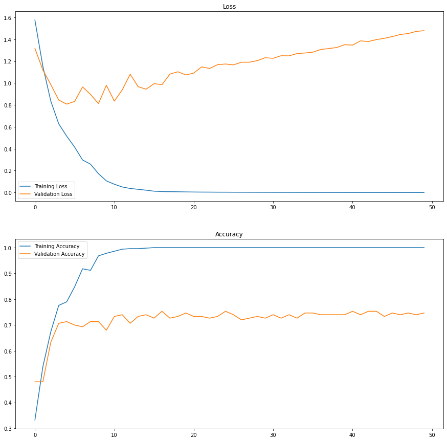
These results are not great. In terms of validation accuracy (bottom orange line), the plot shows that the model learns quickly, but then plateaus by the 5th epoch. It also quickly learns to predict the validation data, reaching 100% accuracy by the 12th epoch. But 100% on the training data is not a good thing if the validation accuracy does not keep pace.
The more important pattern revealed by these graphs is the significant gap between performance on the training and validation sets. This gap means that the model is over-fitting.
That is, the network is learning the features of the training images so well that it cannot see very far beyond them. In other words, it is memorizing the training data, and failing to find the generalizable patterns that would allow it to recognize similar objects in the validation images. This is not good, because it means that in the real world, my Toy Robot will get confused if it sees a Lego that doesn’t perfectly match the images that it was trained on. I want the model to be able to generalize about what makes a Lego a Lego, so that it can recognize a previously unseen Lego from a Bananagram.
In the following sections, I’ll add features to the model that address the overfitting problem, attempting to close the gap between the training and validation accuracy scores. First, let’s take a closer look at what the model sees.
Performance On The Test Set
The model trains only on the training data. The validation data informs this training, because the model saves its progress (its weights and bias values) every time the validation accuracy improves. To get a truly ‘real world’ taste of how the model peforms, however, we can use it to predict on images that it has not seen at all during training - the test set. The model’s accuracy on the test set then, will provide a good metric of how well the many iterations of our model compare to each other.
In the code below, I will:
- Import the required packages for importing the test set images
- Set up the parameters for the predictions
- Load in the saved model file from training
- Create a function for preprocessing the test set images in the same way that training and validation images were
- Create a function for making predictions, returning both predicted class label, and predicted class probability
- Iterate through our test set images, preprocessing each and passing to the network for prediction
- Create a Pandas DataFrame to hold all prediction data
# import required packages
from tensorflow.keras.models import load_model
from tensorflow.keras.preprocessing.image import load_img, img_to_array
import numpy as np
import pandas as pd
from os import listdir

# parameters for prediction
model_filename = 'models/toy_robot_basic_v01.h5'
img_width = 128
img_height = 128
labels_list = ['bananagrams', 'brios', 'cars', 'duplos', 'magnatiles']

# load model
model = load_model(model_filename)

# image pre-processing function
def preprocess_image(filepath):

    image = load_img(filepath, target_size = (img_width, img_height))
    image = img_to_array(image)
    image = np.expand_dims(image, axis = 0)
    image = image * (1./255)

    return image

# image prediction function
def make_prediction(image):

    class_probs = model.predict(image)
    predicted_class = np.argmax(class_probs)
    predicted_label = labels_list[predicted_class]
    predicted_prob = class_probs[0][predicted_class]

    return predicted_label, predicted_prob

# loop through test data
source_dir = 'data/test/'
folder_names = ['bananagrams', 'brios', 'cars', 'duplos', 'magnatiles']
actual_labels = []
predicted_labels = []
predicted_probabilities = []
filenames = []

for folder in folder_names:

    images = listdir(source_dir + '/' + folder)

    for image in images:

        processed_image = preprocess_image(source_dir + '/' + folder + '/' + image)
        predicted_label, predicted_probability = make_prediction(processed_image)

        actual_labels.append(folder)
        predicted_labels.append(predicted_label)
        predicted_probabilities.append(predicted_probability)
        filenames.append(image)

# create dataframe to analyse
predictions_df = pd.DataFrame({"actual_label" : actual_labels,
                               "predicted_label" : predicted_labels,
                               "predicted_probability" : predicted_probabilities,
                               "filename" : filenames})

predictions_df['correct'] = np.where(predictions_df['actual_label'] == predictions_df['predicted_label'], 1, 0)
Thus we have a convenient dataframe storing our test set prediction data (predictions_df). A small sample of those 75 rows in that dataframe looks like this:
| actual_label | predicted_label | predicted_probability | filename | correct |
|---|---|---|---|---|
| bananagrams | bananagrams | 0.65868604 | IMG_7817.jpg | 1 |
| brios | brios | 0.99941015 | b1.jpg | 1 |
| cars | magnatiles | 0.99988043 | c119.jpg | 0 |
| duplos | bananagrams | 0.6900331 | IMG_8532.jpg | 0 |
| magnatiles | magnatiles | 0.994294 | IMG_8635.jpg | 1 |
This data can be used to analyze the model’s performance on specific images in a few different ways:
- Calculate the test set classification accuracy (below).
- Creating a confusion matrix (below).
- Using a Grad-CAM analysis (below).
Test Set Classification Accuracy
To calculate test set classification accuracy:
# overall test set accuracy
test_set_accuracy = predictions_df['correct'].sum() / len(predictions_df)
print(test_set_accuracy)
The baseline network gets 74.7% classification accuracy on the test set. This is the metric I’ll be trying to improve in subsequent iterations.
Test Set Confusion Matrix
Overall Classification Accuracy is useful, but it can obscure where and why the model struggled. Maybe the network is predicting extremely well on Bananagrams, but it thinks that Magnatiles are Brios? A Confusion Matrix can show us these patterns, which I create using the predictions dataframe below.
# confusion matrix
confusion_matrix = pd.crosstab(predictions_df['predicted_label'], predictions_df['actual_label'])
print(confusion_matrix)
# or, with percentages larger dataframes
# confusion_matrix = pd.crosstab(predictions_df['predicted_label'], predictions_df['actual_label'], normalize = 'columns')
# print(confusion_matrix)

actual_label     bananagrams  brios  cars  duplos  magnatiles
predicted_label
bananagrams               10      1     0       0           0
brios                      4     12     0       1           1
cars                       0      1    13       0           0
duplos                     0      0     0      13           6
magnatiles                 1      1     2       1           8
So, while overall our test set accuracy was ~75%, for each individual class we see:
- Bananagrams: 66.7%
- Brios: 80%
- Cars: 86.7%
- Duplos: 86.7%
- Magnatiles: 53.3%
Insightful! I honestly thought the Magnatiles would be the most recognizable, but here the model thinks a big portion of them are Duplos. Perhaps its not surprising since Magnatiles and Duplos share common features. They are both square/blocky and made of solid colors, which combine to form multi-color, multi-block shapes. But that is just me guessing! To see what features the model actually is picking up on, I use a grad-CAM analysis.
Grad-CAM Analysis
Gradient-weighted Class Activation Mapping, or Grad-CAM, is a great way to visualize what the model sees by overlaying the activated features from the last convolutional layer onto the actual image! A heatmap is used to color-code the regions of the image that the model found most useful for classifying it as one thing or another.
In the code below, I:
- Find the name of the last convolutional layer (layers are named and saved in Keras as part of the model object) (Any convolutional layer can be used, but the last one should be the most meaningful)
- Set the image properties and directory paths (as we did when calling test images) (Any image can be analyzed)
- Define the Grad-CAM function to turn activated features into mappable objects (I use a script I found, not fully sure what “tape” and “GradientTape” refer to)
- Define a function to preprocess image(s) to analyze
- Define a function to overlay the heat-map on the images
- Define a function to plot the image and the heatmap
import os
import cv2
import numpy as np
import tensorflow as tf
import matplotlib.pyplot as plt
from tensorflow.keras.models import load_model
from tensorflow.keras.preprocessing.image import load_img, img_to_array

os.chdir("C:/Dat_Sci/Data Projects/Toy Robot")

# Load the model
model_path = 'models/Toy_Robot_basic_v01.h5'
model = load_model(model_path)

# Print all layers in the model to inspect names and shapes
for i, layer in enumerate(model.layers):
    print(i, layer.name, layer.output.shape)

# Find the last Conv2D layer in the model
def find_last_conv_layer(model):
    for layer in reversed(model.layers):
        if isinstance(layer, tf.keras.layers.Conv2D):
            return layer.name
    raise ValueError("No Conv2D layer found in the model.")

# Get the last conv layer name (this is what we will use for Grad-CAM)
last_conv_layer_name = find_last_conv_layer(model)
print("Last conv layer name:", last_conv_layer_name)

# Define which conv layers to use for Grad-CAM (here we just use the last convolutional layer)
conv_layers = [last_conv_layer_name]

# Define image properties and directories
img_size = (128, 128)  # Model input size
test_dir = "data/test"  # Directory with test images
output_dir = "grad_cam"  # Directory to save Grad-CAM images
os.makedirs(output_dir, exist_ok=True)

# Grad-CAM Function
def grad_cam(model, img_array, target_layer_name):
    """Compute Grad-CAM heatmap for a specified convolutional layer."""
    conv_layer = model.get_layer(target_layer_name)

    # Create a model that maps the input image to the conv layer output and predictions
    grad_model = tf.keras.models.Model(
        inputs=[model.input],
        outputs=[conv_layer.output, model.output]
    )

    with tf.GradientTape() as tape:
        conv_output, predictions = grad_model(img_array)
        # Get the predicted class index
        class_idx = tf.argmax(predictions[0])
        # Use the score of the predicted class as the loss
        loss = predictions[:, class_idx]

    # Compute gradients of the loss with respect to the conv layer output
    grads = tape.gradient(loss, conv_output)
    pooled_grads = tf.reduce_mean(grads, axis=(0, 1, 2))

    conv_output = conv_output[0]
    heatmap = np.mean(conv_output * pooled_grads, axis=-1)

    # Normalize the heatmap between 0 and 1
    heatmap = np.maximum(heatmap, 0)
    if np.max(heatmap) != 0:
        heatmap /= np.max(heatmap)

    return heatmap

# Image Preprocessing
def preprocess_image(img_path):
    """Load and preprocess an image for the model."""
    img = load_img(img_path, target_size=img_size)
    img_array = img_to_array(img) / 255.0  # Normalize
    img_array = np.expand_dims(img_array, axis=0)  # Add batch dimension
    return img, img_array

def overlay_heatmap(heatmap, img_path, alpha=0.4):
    """Overlay the Grad-CAM heatmap on the original image."""
    img = cv2.imread(img_path)
    img = cv2.resize(img, img_size)

    heatmap = cv2.resize(heatmap, (img.shape[1], img.shape[0]))
    heatmap = np.uint8(255 * heatmap)
    heatmap = cv2.applyColorMap(heatmap, cv2.COLORMAP_JET)

    # Blend heatmap with the original image
    superimposed_img = cv2.addWeighted(img, 1 - alpha, heatmap, alpha, 0)
    return superimposed_img

# Apply Grad-CAM on Test Images
def run_grad_cam_on_test_set():
    """Run Grad-CAM on test images for specified convolutional layers."""
    for category in os.listdir(test_dir):
        category_path = os.path.join(test_dir, category)
        if not os.path.isdir(category_path):
            continue  # Skip non-directory files

        for img_name in os.listdir(category_path):
            img_path = os.path.join(category_path, img_name)
            try:
                # Preprocess the image
                original_img, img_array = preprocess_image(img_path)

                # Iterate over the chosen conv layers (here, just the last conv layer)
                for layer in conv_layers:
                    heatmap = grad_cam(model, img_array, target_layer_name=layer)
                    superimposed_img = overlay_heatmap(heatmap, img_path)

                    # Save the Grad-CAM output image
                    heatmap_path = os.path.join(output_dir, f"heatmap_{layer}_{category}_{img_name}")
                    cv2.imwrite(heatmap_path, superimposed_img)

                    # Display the original and Grad-CAM images side by side
                    fig, ax = plt.subplots(1, 2, figsize=(10, 5))
                    ax[0].imshow(original_img)
                    ax[0].set_title(f"Original Image ({category})")
                    ax[0].axis("off")

                    ax[1].imshow(cv2.cvtColor(superimposed_img, cv2.COLOR_BGR2RGB))
                    ax[1].set_title(f"Grad-CAM at {layer}")
                    ax[1].axis("off")

                    plt.show()

            except Exception as e:
                print(f"Error processing {img_path}: {e}")

# --- Run Grad-CAM on the Test Set ---
run_grad_cam_on_test_set()
Grad-CAM images offer two important insights, which I’ll call Bias insight and Depth insight,
Bias Insight
First, we can see whether or not the model is picking up on the features that would distinguish one class of object from another. In the first image below, the model seems to have honed in on the Duplo very well, with the most important feature being the top texture with the circular connectors. In the second image, however, we see the opposite, where the model seems to have found the floor around the actual Bananagram as the important feature for classification.
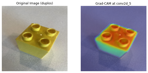
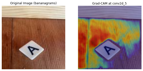
Bias is a pervasive issue in CNN tasks. Bias happens when a model learns to predict on spurious features, something in the data other than the features that would distinguish or separate classes in the real world. Whether or not the model predicted these first two images correctly is not exactly my concern here. We know that if a model focuses on the unique circular connectors of Duplos, it will have a better chance of predicting Duplos that it hasn’t seen before, but if the model can’t recognize a Bananagram from the floor, it probably does not know what actually makes a Bananagram a Bananagram, even if it does guess correctly.
When a model is biased, it is often due to contextual, or background bias. That is, because it has learned to correctly predict on contextual features that are associated with the class in training (i.e., with biased images), but not in real life.
In this case, the model might have predicted the Banagram correctly (it did not, it gave it a 53% chance being a Duplo) if it associated the floor (or perhaps the shape of its cut out) with the class Bananagram. If all my Bananagram images were taken against a wood floor background, and all the Duplos were taken against a white table backdrop, the model could correctly guess the class of each just by identifying the features of the background. This so-called shortcut learning is often the result of such covariate shift. In this particular case, I should be concerned that the Duplo images are biased, since having picked up on the floor not the object, the model chose Duplo instead of Bananagram.
The issue gets more even more complicated when considering class imbalance. If four out of the five classes of images have a 50/50% split in wood floor vs. white table backgrounds, but one class (lets say Bananagrams) has a 70/30% split, the model might still be biased towards that 70% background because all other things being equal, it is at least 70% correct for one class of objects if it identifies the background alone as its defining feature. Further, if is has trouble identifying distinguishing features in the other classes, then it might still guess Bananagram every time it sees a wood floor background. Finally, it may be that the proportion of backgrounds is the same in each class of images, but because Bananagrams are smaller, they take up less space in the frame, and therefore there is more (wood floor) background evident in the class Bananagrams than there is in other classes.
I’ll address bias as a concern with my self-collected data set again in the conclusion.
Depth Insight
Secondly, we can use the grad-CAM images to compare what the model predicted correctly and what it missed! In the images below it looks like the network learned the features of the Magnatiles quite well. The heat-map looks like it is focused on the whole shape, as well as the screws, and the magnets inside the object.
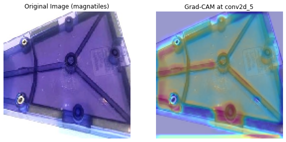
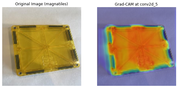
However, while the top image was correctly identified as a Magnatile, the bottom image was identified as a Duplo. This may be a bias issue, but it also seems likely, this time, that the model is simply failing to understand the difference between Magnatiles and Duplos and deep enough level.
In subsequent iterations, I’ll tackle the many issues identified above with various methods that should improve the model’s overall performance.
Model Iterations
Rather than reproduce all of the text and discussion above for each of the subsequent iterations, I’ll describe basic changes and performance metrics in the table below. Then, in the sections that follow, I’ll discuss what additions are made, the rationalle behind them, and the result that matters: test set accuracy.
| Model | Changes Made | Validation Accuracy | Test Accuracy |
|---|---|---|---|
| 1 | Baseline (see above) | 73.3% | 74.7% |
| 2 | Add Dropout (0.5) | 76% | 80% |
| 3 | Add Image Augmentation, no Dropout | 77.3% | 74.7% |
| 4 | Adjusted Learning Rate, w/Dropout & Image Augmentation | 76.7% | 76% |
| 5 | Add 3rd Convolutional Layer (CV1_32, CV2_32, CV3_32, Dense_32), Reduce Dropout (0.25) | 74.7% | 77.3% |
| 6 | Increase Filters in 3rd Layer (CV1_32, CV2_32, CV3_64, Dense_32) | 76.7% | 73.3% |
| 7 | Increase kernel size in 3rd layer (CV1_32, CV2_32, CV3_64 (kernel size = 5x5), Dense_32) | 75.3% | 76% |
| 8 | Add 4th Convolutional Layer, reduce filters in 1st (CV1_16, CV2_32, CV3_64, CV4_64 (kernel size = 3x3), Dense_32) | 80% | 80% |
| 9 | Use MobilenetV2 base model | 100% | 100% |
Overcoming Overfitting With Dropout
Dropout Overview
Dropout is a technique used in Deep Learning primarily to reduce the effects of over-fitting. As we have seen, over-fitting happens when the network learns the patterns of the training data so specifically that it essentially memorizes those images as the class of object itself. Then when it sees the same class of object in a different image (in the validation or test set), it cannot recognize it.
Dropout is a technique in which, for each batch of observations that is sent forwards through the network, a pre-specified portion (typically 20-50%) of the neurons in a hidden layer are randomly deactivated. This can be applied to any number of the hidden layers. When neurons are temporarily deactivated - they take no part in the passing of information through the network.
The math is the same, the network will process everything as it always would (taking the sum of the inputs multiplied by the weights, and adding a bias term, applying activation functions, and updating the network’s parameters using Back Propagation) - but now some of the neurons are simply turned off. If some neurons are turned off, then the other neurons have to jump in and pick up the slack (so to speak). If those other neurons were previously dedicated to certain very specific features of training images, they will now be forced to generalize a bit more. If over-trained neurons that were turned off in one epoch jump back in in the next, they now contend with a model that has found more generalizable patterns and will have to tune accordingly.
Over time, with different combinations of neurons being ignored for each mini-batch of data - the network becomes more adept at generalizing and thus is less likely to overfit to the training data. Since no particular neuron can rely on the presence of other neurons, and the features with which they represent, neurons cannot co-adapt - the network learns more robust features, and are less susceptible to noise.
Implementing Dropout
Adding dropout using Keras is as simple as installing the function and adding a line of code. I saved a new code sheet with the three following changes:
# import
from tensorflow.keras.layers import Dropout

# add dropout to the output layer
# ...
model.add(Dense(num_classes))
model.add(Dropout(0.5))
model.add(Activation('softmax'))
# ...

# save model
model_filename = 'models/toy_robot_dropout_v01.h5'
Results with Dropout
Other than the above, the following output results from the same exact code as our baseline model. Adding dropout was the only change.
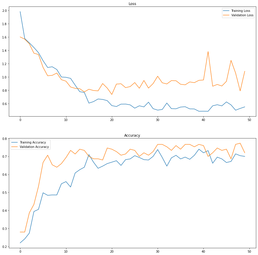
The best classification accuracy on the validation set was 76%, not significantly higher than the 75.3% we saw for the baseline network. Validation set accuracy plateaus early again, at about the 10th epoch.
Accuracy on the test set was 80%, which is a nice bump from the 74.7% test set accuracy from the baseline model.
The model is no longer over-fitting. The gap between the classification accuracy on the training set and the validation set has been eliminated. In fact, the model is consistently predicting better on the validation set, which might indicate that the validation set data is more consistent within each class.
On the other hand, we still see a divergence with respect to training vs. validation loss. This means that even though the network is consistently predicting the validation set at about 72-76%, it becomes less confident in its predictions. Or, it is becoming less confident in the validation set preditions, while its confidence in training predictions plateaus.
Next, I turn to another method for reducing overfitting, Image Augmentation.
Image Augmentation
Image Augmentation Overview
Image Augmentation means altering the training set images in random ways, so that the network will see each image, or feature within it, in a slightly different way each time it is passed through. Because the images are augmented slightly at each pass, the network can no longer memorize them. The aim is to increase the model’s ability to generalize.
Image augmentation in CNN works like an image editor application: we can zoom, rotate, shear, crop, alter the brightness, etc. But instead of doing this manually and adding nuanced versions of each image to our dataset, we simply set the parameters and let Keras randomly alter the images before they’re passed through the training set.
Implementing Image Augmentation
When setting up and training the baseline and dropout models - we used the ImageGenerator function to rescale the pixel values. Now we will use it to add in the Image Augmentation parameters as well. In the code below, we add these transformations in and specify the magnitudes that we want each applied:
# image generators
training_generator = ImageDataGenerator(rescale = 1./255,
                                        rotation_range = 20,
                                        width_shift_range = 0.2,
                                        height_shift_range = 0.2,
                                        zoom_range = 0.1,
                                        horizontal_flip = True,
                                        brightness_range = (0.5,1.5),
                                        fill_mode = 'nearest')

validation_generator = ImageDataGenerator(rescale = 1./255)
# It is important to note that these transformations are applied *only* to the training set, and not the validation set.

# save model
model_filename = 'models/toy_robot_augmented_v01.h5'
- Rotation_range of 20 refers to the maximum degrees of rotation we want. Every time an image is passed, the ImageDataGenerator will randomly rotate it between 0-20 degrees
- Width_shift_range and height_shift_range of 0.2 refer to the maximum width and height that we are happy to shift. The ImageDataGenerator will randomly shift our image up to 20% both vertically and horizonally
- Zoom_range of 0.1 means a maximum of 10% inward or outward zoom
- Horizontal_flip = True means that each time an image flows in, there is a 50/50 chance of it being flipped
- Brightness_range between 0.5 and 1.5 means our images can become brighter or darker
- Fill_mode set to “nearest” means that when images are shifted and/or rotated, we’ll just use the nearest pixel to fill in any new pixels that are required - and it means our images still resemble the scene
Results with Augmentation
As before, I trained the same baseline network architecture, this time only changing the images flowing in.
I dropped Dropout from the model, so the Augmented Image model can be compared to both the baseline model and the dropout model.
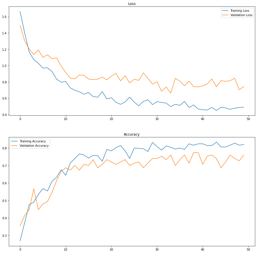
The best classification accuracy on the validation set was 77.3%, slightly higher than the 75.3% we saw for the baseline network. Validation set accuracy plateaus again, but not as early, and its highest validation accuracy was achieved in the 39th epoch.
Accuracy on the test set was 74.7%, same as the 74.7% test set accuracy from the baseline model, and not as good as the 80% accuracy from the Dropout model.
The model appears to be slightly overfitting. Compared to the baseline model, the gap between the classification accuracy on the training set and the validation set has not been eliminated, but it is greatly reduced, which unfortunately in this case did not lead to better performance overall.
Using Image Augmentation and applying Dropout together might be a powerful combination. I’ll do so in later iterations.
Before turning to the model architecture, however, I’ll try to increase the model’s performance by adjusting the learning rate when the performance metrics plateau.
Learning Rate Reduction
Learning Rate Overview
The learning rate in a Convolutional Neural Network refers to how big a step the model takes during gradient descent in its effort to minimize error. For each weight, the model applies gradient descent to find the best value that minimizes the overall loss across all layers. The minima is the point at which a weight’s value acheives minimum loss for the model as a whole. Because image data present complex (not linear) patterns, each weight might positively contribute to the model at different values, but we want it to find the best overall weight value for the entire model, or the global minima, among contending minima. Along the way, the model might encounters local minima, which are suboptimal, or misleading low points that can trap the model’s learning process.
If the gradient descent algorithm moves too quickly, the model risks overshooting the global minima. On the other hand, if it moves too slowly, it risks getting stuck in local minima and never getting out.
Keras’ LearningRateReducer allows us to reduce learning (the rate of gradient descent) in the training process if and when the learning starts to plateau. That is, we can tell the model to slow down if, epoch-to-epoch, it is not making any improvements in terms of accuracy or loss.
Implementing Learning Rate Reducer
Keras’ ReduceLROnPlateau function allows this as a model callback. The code belongs with our other “training parameters”, and is passed in our model.fit() “history” object.
In the code below, I:
- Set it to monitor the validation accuracy
- Decrease speed by 0.5…
- If (patience) Validation Accuracy does not increase in 4 epochs
# install packages
from tensorflow.keras.callbacks import ReduceLROnPlateau

# save as
model_filename = 'models/Toy_Robot_LRreducer_v01.h5'

# reduce learning when validation loss stops improving
reduce_lr = ReduceLROnPlateau(monitor='val_accuracy',  # Monitor validation accuracy
                              factor=0.5,         # Reduce LR by half
                              patience=4,         # Wait 4 epochs before reducing
                              min_lr=1e-6,        # Minimum learning rate
                              verbose=1)          # Print updates
# train the network

history = model.fit(x = training_set,
                    validation_data = validation_set,
                    batch_size = batch_size,
                    epochs = num_epochs,
                    callbacks = [save_best_model, reduce_lr])
Results with Learning Rate Reduction
As before, I trained the same baseline network architecture, this time with both Image Augmentation and Dropout (0.5)
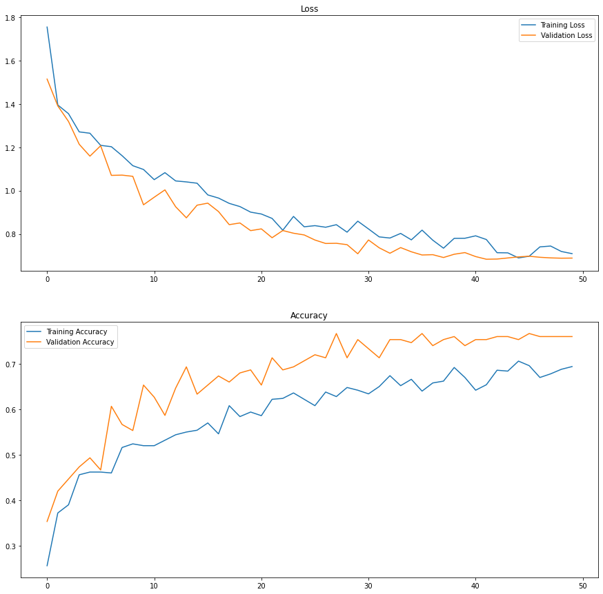
The best classification accuracy on the validation set was 76.7, only slightly higher than 75.3% we saw for the baseline network.
Accuracy on the test set was 76%, also slightly higher than the 74.7% test set accuracy from the baseline model, and not as good as the 80% accuracy from the Dropout model.
The Learning Rate Reducer kicked in first at epoch 18. After which the model slowly improved to find its best validation accuracy at epoch 28. So, the reduction in learning might have helped the model find a more accurate fit. The learning rate changed again at epochs 32, 36, 40, 44, and 48, with no further improvement to the model’s performance.
Instead of overfitting, the model is now underfitting, as evidenced by the higher validation accuracy and lower validation loss, compared to the those metrics on the training set. This is likely due to the combination of both Dropout and Image Augmentation used in this model.
In future iterations, I will scale down the Dropout and Image Augmentation to try to get a better convergence of test and training accuracy. Because the learning rate reduction helped only after its first reduction, I will also lengthen the patience parameter in future models.
Network Architecture
So far, I’ve used the same network archiecture for each of the Baseline, Dropout, Image Augmentation, and Learning Rate models:
- 2 convolutional layers
- Each with 32 filters
- A single Dense layer with 32 neurons
One to figure out if there are better architectures is to use Keras_tuner, a Keras function that automates what I will do below. I plan to use Keras_tuner in Toy Robot 2.0, but for now, I want to lay out what benefits, if any, subtle changes to the model architecture might gain.
First I’ll discuss the parameters, and then I’ll post the results, wholesale.
Convolutional Layers
Convolutional Layers in CNNs detect patterns by filtering the image, or aggregating within small chunks (or, kernels) of the image. The filtering produces a feature map, which is then passed on to the next convolutional layer. Adding convolutional layers, or layer blocks, can help the network detect more complex patterns, but it can also risk overfitting if the model learns the training images too closely.
Below I’ll experiment with adding a third and a fourth convolutional layer. For small data-sets like mine, however, it is usually recommended that fewer layers are better to prevent overfitting.
Filters
There may be any number of filters in a convolutional layer - though we usually assign them in square multiples of the image dimensions. Each filter picks up a distinct pattern, and learns, in training, what patterns are relevant or not. Adding filters to a convolutional layer can help a network find more detailed patterns, but it can also lead to overfitting. Further, more filters means more weights to adjust in training, which means it takes more time for a network to learn.
Below I’ll experiment with increases and decreases of filters in select layers. Again, for small data-sets, less filters is generally recommended.
Kernel Size
The kernel size is the dimension of image space that a filter is combing over and abstracting from. A larger kernel size might capture larger, contextual patterns, but it may also capture noise. Smaller kernels capture finer details, but may miss larger contextual information.
Below I’ll experiment with increasing the Kernel size in one of the layers, but it should be noted that a 3x3 pixel kernel size is standard practice, as it balances detail and efficiency.
Pooling
Pooling layers are usually part of a convolutional layer block. Pooling shrinks the dimensions of the (filtered) image for subsequent convolutional layers, which allow the network to then filter more abstract features. Pooling helps to reduce overfitting, but too much pooling can lead to losing information that relate to important features.
Max Pooling is the standard technique, although other pooling methods can be used, such as Global Average Pooling. I will not experiment with other pooling methods here.
Other architecture parameters can be changed or added, including:
- Stride: how many pixels each filter moves at a time as it moves across the image. The default stride in Keras is 1.
- Activation Function: Applied to each layer - tells each neuron whether or not (and how) to send information (weight value) to the next layer. I use the Relu (or Rectified Linear Unit) activation function here, which I’ve seen to be most common. It works by passing information neuron to neuron only if the weights reach a threshold positive value.
- Batch Normalization: Scales weight values 0-1 (usually before being activated) for every batch, usually once per convolutional layer. Although it is a standard practice to include Batch Normalization to stabilize training, I’ve found that the time costs are not worth the results.
Architecture Experiment 1
For the first experiment, I modify the previous learning parameters, and add one identical convolutional layer. In the code below, I only include what is changed so as to avoid long blocks of redundant information:
# Decrease Image Augmentation
training_generator = ImageDataGenerator(
    rescale=1./255,
    rotation_range=15, # Reduce rotation
    width_shift_range=0.15,  # Reduce shift (was 0.2)
    height_shift_range=0.15,
    zoom_range=0.15,  # Keep small zoom (was 0.2)
    horizontal_flip=True,  # Keep flipping
    shear_range=10, # add shearing
    brightness_range=(0.8, 1.3),  # Less extreme brightness (was 0.5–1.5)
    fill_mode='nearest'
)

# Add 3rd Convoluational Layer
model.add(Conv2D(filters = 32, kernel_size = (3,3), padding = 'same'))
model.add(Activation('relu'))
model.add(MaxPooling2D())

# Decrase Dropout
# output layer
model.add(Dense(num_classes))
model.add(Dropout(0.25))
model.add(Activation('softmax'))

# Save model as...
model_filename = 'models/Toy_Robot_tuned_v01.h5'

# Increase learning patience
reduce_lr = ReduceLROnPlateau(monitor='val_accuracy',  # Monitor validation loss
                              factor=0.5,         # Reduce LR by half
                              patience=5,         # Wait 3 epochs before reducing
                              min_lr=1e-6,        # Minimum learning rate
                              verbose=1)          # Print updates

# Summary
model.summary()
_________________________________________________________________
Layer (type)                 Output Shape              Param #
=================================================================
conv2d_2 (Conv2D)            (None, 128, 128, 32)      896
_________________________________________________________________
activation_4 (Activation)    (None, 128, 128, 32)      0
_________________________________________________________________
max_pooling2d_2 (MaxPooling2 (None, 64, 64, 32)        0
_________________________________________________________________
conv2d_3 (Conv2D)            (None, 64, 64, 32)        9248
_________________________________________________________________
activation_5 (Activation)    (None, 64, 64, 32)        0
_________________________________________________________________
max_pooling2d_3 (MaxPooling2 (None, 32, 32, 32)        0
_________________________________________________________________
conv2d_4 (Conv2D)            (None, 32, 32, 32)        9248
_________________________________________________________________
activation_6 (Activation)    (None, 32, 32, 32)        0
_________________________________________________________________
max_pooling2d_4 (MaxPooling2 (None, 16, 16, 32)        0
_________________________________________________________________
flatten_1 (Flatten)          (None, 8192)              0
_________________________________________________________________
dense_2 (Dense)              (None, 32)                262176
_________________________________________________________________
activation_7 (Activation)    (None, 32)                0
_________________________________________________________________
dense_3 (Dense)              (None, 5)                 165
_________________________________________________________________
dropout_1 (Dropout)          (None, 5)                 0
_________________________________________________________________
activation_8 (Activation)    (None, 5)                 0
=================================================================
Total params: 281,733
Trainable params: 281,733
Non-trainable params: 0
AE 1 Results:
- Validation Accuracy: 74.7%
- Test Accuracy: 77.3%
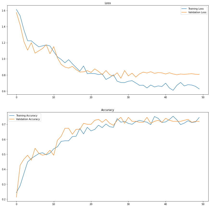
Training and Validation Accuracy seem to be converging nicely here, which is good news for our training parameters. However, the training loss is now slightly outpacing the validation loss. I’ll experiment with a filter number change before adjusting training parameters again.
Architecture Experiment 2
Increasing number of filters in the 3rd Convolutional Layer from 32 to 64:
Layer (type)                 Output Shape              Param #
=================================================================
conv2d_8 (Conv2D)            (None, 128, 128, 32)      896
_________________________________________________________________
activation_14 (Activation)   (None, 128, 128, 32)      0
_________________________________________________________________
max_pooling2d_8 (MaxPooling2 (None, 64, 64, 32)        0
_________________________________________________________________
conv2d_9 (Conv2D)            (None, 64, 64, 32)        9248
_________________________________________________________________
activation_15 (Activation)   (None, 64, 64, 32)        0
_________________________________________________________________
max_pooling2d_9 (MaxPooling2 (None, 32, 32, 32)        0
_________________________________________________________________
conv2d_10 (Conv2D)           (None, 32, 32, 64)        18496
_________________________________________________________________
activation_16 (Activation)   (None, 32, 32, 64)        0
_________________________________________________________________
max_pooling2d_10 (MaxPooling (None, 16, 16, 64)        0
_________________________________________________________________
flatten_3 (Flatten)          (None, 16384)             0
_________________________________________________________________
dense_6 (Dense)              (None, 32)                524320
_________________________________________________________________
activation_17 (Activation)   (None, 32)                0
_________________________________________________________________
dense_7 (Dense)              (None, 5)                 165
_________________________________________________________________
dropout_3 (Dropout)          (None, 5)                 0
_________________________________________________________________
activation_18 (Activation)   (None, 5)                 0
=================================================================
Total params: 553,125
Trainable params: 553,125
Non-trainable params: 0
AE 2 Results:
- Validation Accuracy: 76.7%
- Test Accuracy: 73.3%
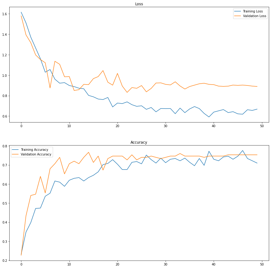
Doubling the number of filters in the 3rd convolutional layer does not seem to have benefited the model’s performance. We can see from the graphs that the model reached its highest validation accuracy somewhat early, and it did not improve after the 15th epoch.
Next I’ll try increasing the kernel size.
Architecture Experiment 3
Increasing kernel size in third layer:
_________________________________________________________________
Layer (type)                 Output Shape              Param #
=================================================================
conv2d_5 (Conv2D)            (None, 128, 128, 32)      896
_________________________________________________________________
activation_9 (Activation)    (None, 128, 128, 32)      0
_________________________________________________________________
max_pooling2d_5 (MaxPooling2 (None, 64, 64, 32)        0
_________________________________________________________________
conv2d_6 (Conv2D)            (None, 64, 64, 32)        9248
_________________________________________________________________
activation_10 (Activation)   (None, 64, 64, 32)        0
_________________________________________________________________
max_pooling2d_6 (MaxPooling2 (None, 32, 32, 32)        0
_________________________________________________________________
conv2d_7 (Conv2D)            (None, 32, 32, 64)        51264
_________________________________________________________________
activation_11 (Activation)   (None, 32, 32, 64)        0
_________________________________________________________________
max_pooling2d_7 (MaxPooling2 (None, 16, 16, 64)        0
_________________________________________________________________
flatten_2 (Flatten)          (None, 16384)             0
_________________________________________________________________
dense_4 (Dense)              (None, 32)                524320
_________________________________________________________________
activation_12 (Activation)   (None, 32)                0
_________________________________________________________________
dense_5 (Dense)              (None, 5)                 165
_________________________________________________________________
dropout_2 (Dropout)          (None, 5)                 0
_________________________________________________________________
activation_13 (Activation)   (None, 5)                 0
=================================================================
Total params: 585,893
Trainable params: 585,893
Non-trainable params: 0
_________________________________________________________________
AE 3 Results:
- Validation Accuracy: 75.3%
- Test Accuracy: 76%
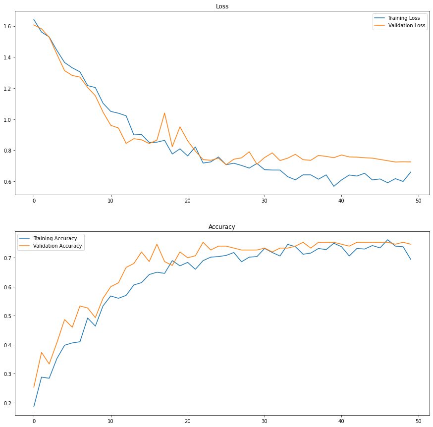
Increasing the kernel size in the third layer did not help my model, although the seems to be learning at steadier rate, as shown by the converging validation and loss metrics. In the next iteration, I’ll change the kernel size back to 3x3, and experiment with layers and filters again.
Architecture Experiment 4
So far adding a layer and increasing filters has not done much to improve the model’s performance. I’ll experiment one more time, decreasing filters in the first layer, and increasing filters in the second layer.
_________________________________________________________________
Layer (type)                 Output Shape              Param #
=================================================================
conv2d (Conv2D)              (None, 128, 128, 16)      448
_________________________________________________________________
activation (Activation)      (None, 128, 128, 16)      0
_________________________________________________________________
max_pooling2d (MaxPooling2D) (None, 64, 64, 16)        0
_________________________________________________________________
conv2d_1 (Conv2D)            (None, 64, 64, 32)        4640
_________________________________________________________________
activation_1 (Activation)    (None, 64, 64, 32)        0
_________________________________________________________________
max_pooling2d_1 (MaxPooling2 (None, 32, 32, 32)        0
_________________________________________________________________
conv2d_2 (Conv2D)            (None, 32, 32, 64)        18496
_________________________________________________________________
activation_2 (Activation)    (None, 32, 32, 64)        0
_________________________________________________________________
max_pooling2d_2 (MaxPooling2 (None, 16, 16, 64)        0
_________________________________________________________________
conv2d_3 (Conv2D)            (None, 16, 16, 64)        36928
_________________________________________________________________
activation_3 (Activation)    (None, 16, 16, 64)        0
_________________________________________________________________
max_pooling2d_3 (MaxPooling2 (None, 8, 8, 64)          0
_________________________________________________________________
flatten (Flatten)            (None, 4096)              0
_________________________________________________________________
dense (Dense)                (None, 32)                131104
_________________________________________________________________
activation_4 (Activation)    (None, 32)                0
_________________________________________________________________
dense_1 (Dense)              (None, 5)                 165
_________________________________________________________________
dropout (Dropout)            (None, 5)                 0
_________________________________________________________________
activation_5 (Activation)    (None, 5)                 0
=================================================================
Total params: 191,781
Trainable params: 191,781
Non-trainable params: 0
AE 4 Results:
- Validation Accuracy: 80%
- Test Accuracy: 80%
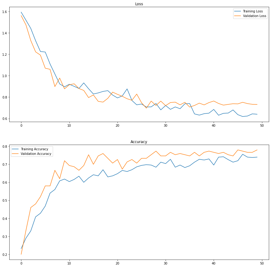
Adding a fourth convolutional layer and changing filters - 16 in the first, and now with 2 convolutional layers of 64 filters - seems to have given our model a little bump in performance. In fact, it is encouraging to see that the model is steadily learning throughout the 50 epochs (although slowly). Running this same model for more epochs might lead to further improvements.
print(confusion_matrix)
actual_label     bananagrams  brios  cars  duplos  magnatiles
predicted_label
bananagrams               12      3     0       0           0
brios                      2     11     0       1           0
cars                       0      1    15       0           2
duplos                     0      0     0      11           2
magnatiles                 1      0     0       3          11
The confusion matrix shows that the current model is now fairly consistent within categories, whereas the baseline model really struggled with Magnatiles. It is perfect in its predictions of Cars on the test set, and much better and predicting Magnatiles, although slightly worse at predicting Brios.
While these results are encouraging, I’ll end my experiments here for now. In future versions of this project, I’ll compare Keras_tuner results with this current model architecture.
Next, I’m eager to see what other CNN models - which have been trained on much larger datasets, and can predict many more classes of images - can do with my Toy Robot task. ___
Transfer Learning With MobiltnetV2
Transfer Learning Overview
Transfer Learning means using a pre-built, pre-trained neural network, and applying it to another specific Deep Learning task. It consists of taking features learned on one problem to solve a new, similar problem.
For image based tasks this means using all the pre-learned convolutional filter values and feature maps from a large network, and instead of using it to predict what the network was originally designed for, piggybacking it, and training it again for another task.
One such pre-trained, large network, is MobileNetV2. MobileNetV2 was developed by Google in 2018, for the purpose creating a ‘lightweight’ CNN architecture that can be used in applications on smaller devices like iphones. Its architecture is slightly different than what I have layed out above, using techniques - depthwise convolutions and inverted residuals - that reduces the number of trainable parameters to efficiently extract image features. It also uses a linear (as opposed to relu) activation function to preserve fine-grained information between layers.
Other pretrained networks are available in Keras’ Applications library. At this point, it is not my purpose to compare them all, so much as it is to compare what a larger, pre-built network like MobilenetV2 can do for my limited dataset.
Implementing MobileNetV2
Again, the Keras functionality makes transfer learning easy in Python, but there are some caveats in the way we set up our model to infer from pretrained features. I’ve learned to use Global Average Pooling in the place of the Flatten layer, and add Batch Normalization to stabilze training. The affect of these tweaks may be left to experiment, but I’ll be sure to include them here. Otherwise, training this model is as simple as:
- Import MobileNetV2
- Define our “base” model as the MobileNetV2 network
- Make its existing weights and biases untrainable
- Add our Dense and Output layers as we would otherwise
- Compile the Model as we would otherwise
# Import
from tensorflow.keras.applications import MobileNetV2

# Load Pretrained Model
base_model = MobileNetV2(weights='imagenet', include_top=False, input_shape=(img_width, img_height, 3))
base_model.trainable = False  # Freeze base layers

# Build Model
model = Sequential([
    base_model,
    GlobalAveragePooling2D(),  # Prefered in Transfer Learning, Preserves spatial relationships better than Flatten()
    BatchNormalization(), # Helps to stabilize training
    Dense(32, activation='relu'),
    Dropout(0.5),
    Dense(5, activation='softmax')
])

# Compile Model
model.compile(loss = 'categorical_crossentropy',
              optimizer = 'adam',
              metrics = ['accuracy'])

# View Model Summary
model.summary()
_________________________________________________________________
Layer (type)                 Output Shape              Param #
=================================================================
mobilenetv2_1.00_128 (Functi (None, 4, 4, 1280)        2257984
_________________________________________________________________
global_average_pooling2d_2 ( (None, 1280)              0
_________________________________________________________________
batch_normalization_2 (Batch (None, 1280)              5120
_________________________________________________________________
dense_6 (Dense)              (None, 32)                40992
_________________________________________________________________
dropout_3 (Dropout)          (None, 32)                0
_________________________________________________________________
dense_7 (Dense)              (None, 5)                 165
=================================================================
Total params: 2,304,261
Trainable params: 43,717
Non-trainable params: 2,260,544
_________________________________________________________________
MobileNetV2 Results:
Validation Set Accuracy: 100% Test Set Accuracy: 100%
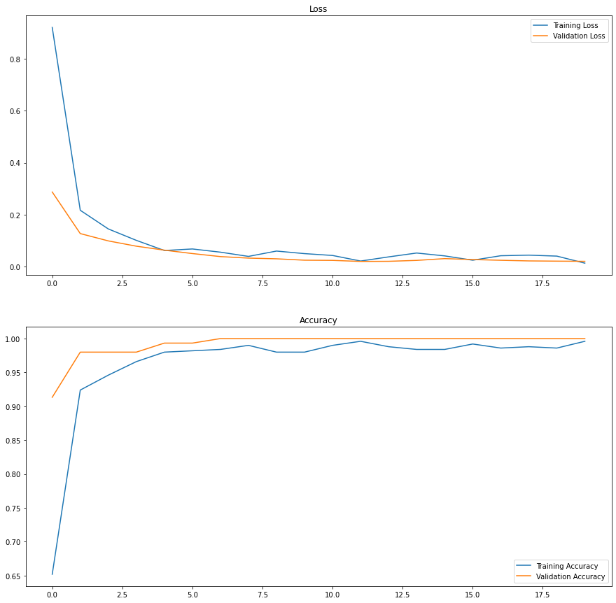
I only ran the MobileNet model for 20 epochs. It achieved 100% Validation accuracy by the 7th epoch. It is hard to argue with 100 percent accuracy.
Overall Results Discussion
After only modest improvements in my self-built model, there were stark improvements when implementing transfer learning with MobileNetV2.
In terms of Classification Accuracy on the Test Set, we saw:
- Baseline Network: 75%
- Baseline + Dropout: 80%
- Baseline + Image Augmentation: 77%
- Baseline + Dropout + Image Augmentation + Learning Rate Reducer: 74%
- Best Architecture + Dropout + Image Augmentation + Learning Rate Reducer: 80%
- Transfer Learning Using MobileNetV2: 100%
Tranfer Learning with MobileNetV2 was a big success. It was able to learn the features in my training data and map them to my validation and test set data with 100% accuracy, and in only 7 epochs of training.
On the other hand, I was frustrated that the adjustments that I made to my own model did not lead to a more improvements.
Growth & Next Steps
The proof of concept was successful. I have shown that I can get very accurate predictions for what bins my kid’s toys belong in, albeit on a small number of classes, but also with a very limited data set. Should this Toy Robot proceed to the next phase of development, I’ll know that I can always employ MobileNetV2 to get accurate predictions.
On the other hand, the process has left me more curious about building a CNN of my own, and I have two ambitions for future versions of this project.
-
Use Keras_tuner: Keras Tuner is available for optimizing the many levers and buttons that make CNNs work. I did not try it here in part because it is time intensive (it works like I have here, making one change at a time, but allows for a greater range of learning and architectural parameters), but mostly because I wanted to see for myself how varying the details of the network architecture can change its performance. I found that it didn’t change much, but there is some hope that adding layers and filters does make a difference, even though for small data sets, it is generally recommended that “less equals more.”
-
Get Scientific about the Data: CNN in Data Science is usually treated as an exercise in optimizing algorithms for the data that is already at hand, and that is how I have approached it here. But one aspect that has not been optimized in this project so far is the images themselves! Earlier I said that I was systematic about the images, but I’ll amend that here to say I was quasi-systematic. I balanced the classes; I aimed to balance the backgrounds within the classes; I aimed to balance closeup, cropped images with distant ones, etc. But I started by taking images of toys strewn - as if haphazardly - across the floor in an effort to mimic real world scenarios. If a Toy Robot can’t see toys as they exist in my house, I thought, what chance does it have to put them in the right bins? But it occured to me that while this impulse is correct for test set data, training and validation data should be easier to differentiate. In fact, they should be taken for the purpose of teaching the model to recognize the specific features that would allow it to differentiate one class from another in the wild. Key identifying features should be emphasized in training images, not burried. Care should also be taken to minimize bias, however. Some image datasets include real-world photographs alongside drawings, while others appear to have been carefully curated in laboratory like settings to minimize the effect of lighting or background bias. More data is better for generalization, although it takes more time to train. The 500 training images I used here make a decidedly “small” dataset. Before I add more images to my Toy Robot dataset for further development, I will carefully study best practices for creating image data sets.