Fantasy BBall Rankings using SHAW-Percentage Transformations
In this project I extract, transform, and load NBA player data for my own fantasy basketball ranking app. I construct a series of ranking algorithms premised on the hypothesis that standard ranking systems scale percentage category scores inaccurately. Existing algorithms typically weight percentage categories linearly by attempts. However, because percentages are bound between 0 and 1, the actual affect of attempts on a player’s percentage is asymptotic - not linear. I develop a Sigmoid-Heuristic-Attempt-Weighting (SHAW) transformation that adjusts for this non-linearity. I then apply this transformation to create six unique fantasy basketball ranking algorithms, which I then systematically compare to each other and to leading platform rankings: ESPN, Yahoo, and Basketball Monster.
Contents
- 00. Project Overview
- 01. Extract Data
- 02. Transformation
- 03. Comparing Rankings with Top-N Player Matchups
- 04. VORP
- 05. Streamlit User Endpoint
- 06. Discussion & Conclusion
Project Overview
Fantasy sports are a popular past time with over 62.5 million participants in the U.S. and Canada (FSGA.org), 20 million of whom regularly play fantasy basketball. In a fantasy sports league, participants (or, team managers) create a fantasy team by competitively drafting from a pool of professional players, whose real game stats become their own fantasy stats for the season. Choosing a successful team requires knowing the players and understanding the league’s scoring format. In 9-category fantasy basketball leagues (the standard competitive fantasy basketball format), teams are compared – and thus players must be evaluated - across nine different measures. To make this easier, the major platforms Yahoo.com and ESPN include player rankings to help managers make their choices. As some critics point out, however, Yahoo and ESPN often include questionable players in their top ranks, and unfortunately, neither platform is exactly transparent about how their rankings are calculated. As a regular fantasy basketballer and data science enthusiast, I join a small but growing literature offering alternatives for better ranking accuracy.
Literature Review
The standard approach to ranking players involves standardizing the scoring categories and then ranking the sum of the players’ Z-Scores (with caveats for percentage categories). But standardization is criticized for over- or under-valuing outliers if distributions are skewed (which they are in the NBA). Victor Wembanyama’s Z-score of 8 in the Blocks category, for example, statistically represents a nearly impossible occurrence when assuming normal distributions, and therefore, the criticism goes, the ranking logic must be inaccurate.
In a recent Medium article, Giora Omer offers an alternative Min-Max normalization approach, which would preserve the relative distribution of each category, without over- or under-valuing the outliers. But while the general approach is discussed, 0-1 scaled rankings are neither demonstrated nor compared. Josh Lloyd at Basketball Monster recently promised an improvement using his DURANT method (Dynamic Unbiased Results Applying Normalized Transformations), which, although inspiring comments like, “Josh Lloyd is trying to crack the fantasy Da Vinci code!”, remains opaque. Lloyd points out that percentage stats seem to vary differently than other, ‘counting stats,’ but does not explicitly offer a method to approach them differently. A Reddit user recently offered a so-called CARUSO method, which promises to use ML for custom category transformations, but how so remains a mystery, and as some readers note, the resulting rankings are not face-valid. The only ranking method that I have seen fully described is Zach Rosenof’s G-Score method, which improves on Z-Score rankings by accounting for period-level (i.e., week-to-week) variance in category accumulation; because some categories are more volatile, investing in them presents risks. Rosenof’s is also the only paper to compare different metrics, finding empirical support for his G-Score rankings method in simulated head-to-head matchups against hypothetical teams using Z-Score rankings.
Actions
Here, I develop and describe six different ranking algorithms of my own and compare them head-to-head against ESPN, Yahoo.com, and Basketball Monster. Each of my ranking methods applies a sigmoid weight to shot-attempts for percentage category transformations (hence SHAW: Sigmoid-Heurisitc Attempt-Weight - transformations). This approach aims to reduce distortion from outliers and enhance the signal from players contributing efficiently across counting categories, but whom are unfairly punished or rewarded in percentage categories. The lambda parameter in the sigmoid function is dynamically tied to the skew of attempts, and its sensitivity is a function of attempt CoV, thus creating a context-sensitive weighting mechanism. From there, my algorithms follow some familiar and some novel ideas.
Table: Summary of SHAW ranking algorithms
| Ranking Algorithm | Description | Strengths | Weaknesses |
|---|---|---|---|
| SHAW-Z | Sum of standardized counting stats and sigmoid weighted percentages | Preserves category dispersion while setting category distributions to like terms | May over-value outliers |
| SHAW-mm | Sum of Min-Max (0-1) scaled counting stats and sigmoid weighted percentages | Preserves category dispersion without overvaluing outliers | May under-value real differences |
| SHAW-Scarce-mm | SHAW-mm ranking with weights applied to scarce categories | Rewards scarce category producers | Scarce categories might also vary unstably from week to week |
| SHAW-rank-sum | Reverse-ranked sum of each-category ranks (using sigmoid weighted percentages) | Simple math; preserves relative player position in each category | Does not account for category variance |
| SHAW-H2H-each | Ranked sum of individual-player categories won vs. the field (using sigmoid weighted percentages) | Rewards balance across categories | Does not account for category variance |
| SHAW-H2H-most | Ranked sum of individual-player matchups won vs. the field (using sigmoid weighted percentages) | Rewards consistency in top categories | Does not account for category variance |
| SHAW-AVG | Average of SHAW-Z and SHAW-Scarce-mm rankings | Aims for robustness | Is difficult to interpret, if not convoluted |
Rankings are then compared using a top-n players ‘super-team’ for each ranking, comparing teams head-to-head across the nine, standard categories.
Along the way, I build an ETL (Extract, Transform, Load) pipeline that starts with up-to-date NBA player stats and ends with an interactive player-ranker dashboard.
Results
I find muted support for my SHAW-transformation rankings. In a top-20 players ‘league’ that includes a Traditional Z-Score ranking with each of the SHAW-rankings, SHAW rankings performed very well against Traditional Z-Score, ESPN, and Yahoo rankings.
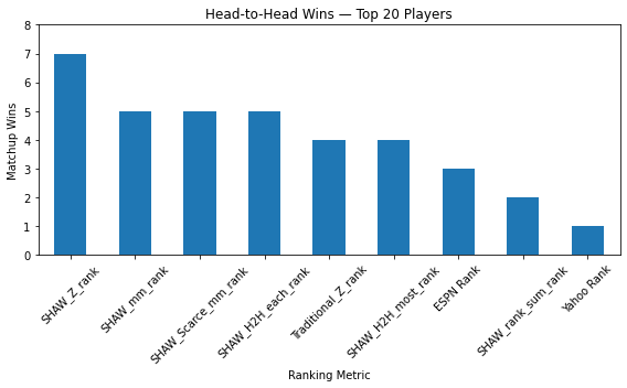
As I’ll demonstrate later, however, in a league that included Basketball Monster (BBM) rankings and further top-n depths (i.e., top 50, top-100 players, etc.), SHAW rankings continued to perform well, but not better than BBM and Traditional Z rankings. In fact, I find that across top n levels, rankings metrics are intransitive: in a top-50 matchup, for example, the winning ranking might be the same that finishes last in the top-60 matchup. Meanwhile, in any matchup at any level, because 9 categories are at stake, Team A might beat Team B and Team B might beat Team C, but Team C beats Team A. Further category wins and matchup wins do not neatly correspond. Nevertheless, the relatively strong performance of SHAW transformations should be a relevant contribution to the growing literature on this topic, and a site for further investigation.
Growth/Next Steps
Although my conclusions regarding the import of SHAW transformations are muted at this point, the project also demonstrates:
- Building and deploying a useful, marketable ETL pipeline
- A solid grasp of statistical tools and transformations
- An ability to think critically about and beyond existing data structures
- A first-of-its-kind empirical ranking algorithms comparison
As such, I am happy to have found a fun project to put my data and research skills together. However, this project can be taken much, much further, and I intend to keep building it out in the future, focusing on the following:
- Continuing empirical research
- Experimenting with weight adjustments in Percentage and Counting categories
- Simulating weekly matchup to observe short term category variances (c.f., Rosenof 2024)
- Scaling up the user endpoint
- Adding 8, 10, and 11 category rankings
- Adding Season Total stats
Extract
I use the NBA API. An unofficial but widely used source for up-to-date NBA statistics.
from nba_api.stats import endpoints
from nba_api.stats.endpoints import LeagueDashPlayerStats
import pandas as pd
import os

os.chdir("C:/...Projects/NBA")

season = "2024-25"

def fetch_player_stats():
    player_stats = LeagueDashPlayerStats(season=season)
    df = player_stats.get_data_frames()[0]  # Convert API response to DataFrame
    return df

nba_24_25 = fetch_player_stats()

nba_24_25.to_csv("data/nba_2024_25.csv", index=False)
The code above returns a dataframe of 66 statistical columns and 550+ rows (players), which get added every time a new players sees the court in the season.
Table: Sample of raw NBA player data
| Player Name | GP | FGA | FGM | REB | AST | TOV | STL | BLK | PTS |
|---|---|---|---|---|---|---|---|---|---|
| LeBron James | 62 | 1139 | 583 | 506 | 525 | 238 | 58 | 35 | 1521 |
| Nikola Jokic | 63 | 1226 | 706 | 806 | 647 | 206 | 109 | 43 | 1845 |
| Victor Wembanyama | 46 | 857 | 408 | 506 | 168 | 149 | 52 | 176 | 1116 |
| Jordan Goodwin | 20 | 104 | 50 | 77 | 29 | 16 | 23 | 11 | 130 |
Transformations
In a typical (category) fantasy basketball league, a team’s weekly score is the sum of players’ cumulative stats in each of the following 9 categories:
- Field Goal Percentage (FG_PCT = FGM/FGA)
- Free Throw Percentage (FT_PCT = FTM/FTA)
- Points (PTS)
- 3-point Field Goals made (FG3M)
- Rebounds (REB)
- Assists (AST)
- Steals (STL)
- Blocks (BLK)
- Turnovers (TOV) (which count negatively)
From there, category leagues can keep score one of two ways: a weekly ‘head-to-head’ matchup win against another team (for the team that wins the most categories), or a win for each category (with all nine categories at stake). Leagues can be customized to include more or less categories, but the default is nine, and the main platforms’ rankings are based on these categories, so that is what I focus on in this write-up. Separately, I also go on to construct rankings based on my own 11-category leauge, which includes 3-Point Feild Goal Percent and Double-Doubles. I’m interested in the following columns:
nba_subset = nba_24_25[['PLAYER_NAME', 'GP', 'FGA', 'FGM', 'FTA', 'FTM', 'FG3M',
             'REB', 'AST', 'TOV', 'STL', 'BLK', 'PTS', 'FG_PCT', 'FG3_PCT', 'FT_PCT']].copy()
The goal is to turn raw NBA statistics into a single player ranking metric that will help team managers understand a single player’s relative fantasy value. It would be easy if there was one statistical category to keep track of – players would be ranked by the number of points they get, for example. (In fact, Points leagues are an alternative scoring format that assigns every statistical category a uniform ‘point’ value, which is too easy to be any fun.) But category leagues require comparisons across 9 different measures. How can you value a player that gets a lot of points and few rebounds vs. one that gets a lot of rebounds and few assists? How do you compare a player that shoots an average free throw percentage on high volume, to a player that shoots above average on low volume?
Before we get into that, it is important to understand the distributions.
Distributions
Most NBA stat categories are positively skewed. Few players get the most points, rebounds, assists, etc.
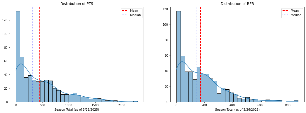
At the same time, a large number of players accumulate very little, if any, stats at all. This fact is important, although it is rarely considered among the experts, and the resulting distributions can change dramatically depending on how we handle it. Ideally, the relative value of a player for fantasy purposes should be considered only in relation to other plausible options, and not in relation to the bulk of players that get little or no playing time. Before making any transformations, thus, a cut-off should be levied, and I define mine at the 25th percentile of games played. Granted, this number is arbitrary, but it is a useful starting point that has the effect of eliminating most ‘garbage time’ players as well as those with season defining injuries (e.g., Joel Embiid in 24-25).
Then, I scale raw category accumulations by games played. Most fantasy relevant players will miss some time during a season due to minor injuries, so using per-game statistics (which is standard) helps to level the field.
# Set Games Played threshold for counting stats
minimum_games_threshold_quantile = 0.25
min_games = stats["GP"].quantile(minimum_games_threshold_quantile)

pg_stats = stats[stats["GP"] >= min_games].copy()

# reverse code turnovers
pg_stats['tov'] = pg_stats['TOV'].max() - pg_stats['TOV']

raw_categories = ['FGA', 'FGM', 'FTA', 'FTM', 'FG3M', 'PTS',
             'REB', 'AST', 'STL', 'BLK', 'tov']

for cat in raw_categories:
    pg_stats[cat + "_pg"] = pg_stats[cat] / pg_stats['GP']
The result is a more modest 400 + player pool, with the large number of zeros eliminated. Distributions are still positively skewed, but there is now some semblance of a tail on the negative end.
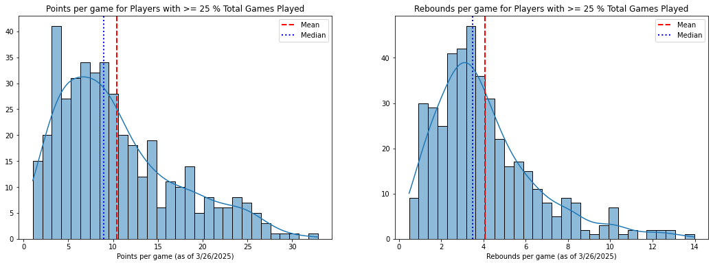
Typically, then the categories are standardized (which I will do in a later section): a players’ Z-score in a category is their difference from the average divided by the standard deviation. Thus, we can compare Points and Rebounds here in like terms. A player that scores 2 standard deviations above the average in points, is comparable to a player that scores 2 standard deviations above the average in Rebounds.
Percentages
Percentage categories deserve special treatment because they are a function of two distributions: makes and attempts. We don’t simply add percentages like we do the other categories: we divide total team makes by total team attempts to get a final percentage score for each weekly matchup.
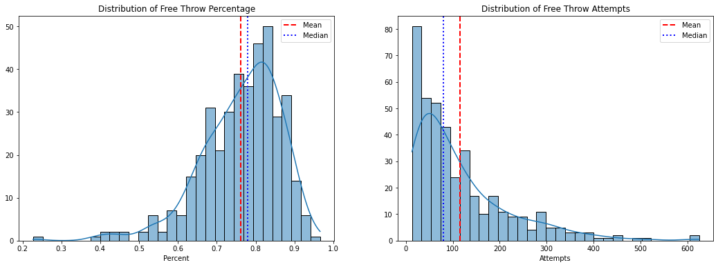
A player that shoots an average percentage on high volume of attempts has a larger impact on a fantasy matchup than an above average shooter that rarely shoots. To evaluate a player’s value in a percentage category, thus, shot volume needs to be considered alongside percent made. The recieved method for doing this is to measure a player’s impact by finding the difference between their number of makes and what is expected given their number of attempts and league percentage averages. Standardizing the impact thus gives a comparable value for that category. For example:
league_pct = pg_stats["FTM"].sum() / pg_stats["FTA"].sum()
FT_impact = pg_stats["FTM"] - (pg_stats["FTA"] * league_pct)
At first glance this would seem fair, a player’s percentage impacts a team’s total to the extent that they take above or below average shot attempts. But because attempts are positively skewed, and percentages are negatively skewed, this method can produce some extreme numbers in both tails. Standardizing yeilds the following Z-Score distribution:
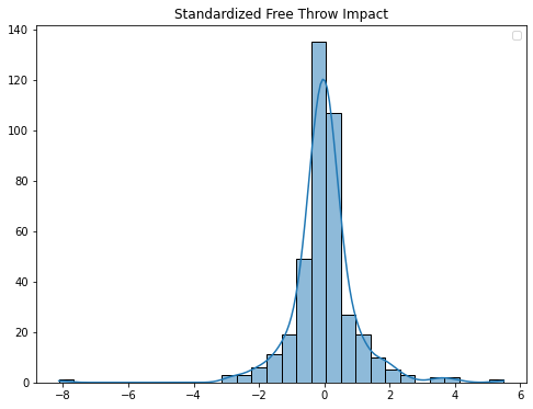
The test case here is Giannis Antetokounmpo. He shoots a sub-par 60% (the league average is 78.2%), but he is also a league-leader in attempts (as an elite scorer otherwise, he gets fouled a lot). Giannis’s Free Throw Z-Score is -8.
Table: Select Players’ Free Throw Percentages, Attempts and standardized Impact score
| Player Name | FT % | FTM | FTA | FT Impact Z Score |
|---|---|---|---|---|
| Giannis Antetokounmpo | 60.2 | 369 | 613 | -8.12 |
| Steph Curry | 92.9 | 252 | 234 | 2.73 |
| Shae Gilgeous-Alexander | 90.1 | 563 | 625 | 5.50 |
| James Harden | 87.4 | 515 | 450 | 3.51 |
| LeBron James | 76.8 | 289 | 222 | -0.23 |
Giannis is an outlier. We can see from the FT Impact Z scores distribution that his -8 is far out in the tail, almost twice as far as the next lowest data point. Imagine now that when we sum a player’s category Z-scores and rank them, Giannis would have a -8.12 in one of the categories, and so his overall score, and therefore his rank, is greatly reduced. To put this -8 in perspective, the average sum of Z-scores for a player in the top 150 is about 7. A critical question for fantasy category valuations is thus, does Giannis hurt you THAT much? On the other side of the distribution, does Shae Gilgeous Alexander’s 90% on high volume help you that much?
For other, counting statistics, I will argue later that skewed distributions are meaningful and useful, but because a percentage statistic is bound between 0 and 1, any positive and negative constributions to it are limited: they are asymptotic, not linear! The graph below visualizes this relationship. Here we can see the league average (78.2), SGA’s (90.1) and Giannis’s (60.2) Free Throw Percentages. The solid lines represent the real impact of each on a hypothetical, average fantasy team for one fantasy week (i.e., the duration of a matchup) when contributing 15 to 150 shots for the team. As their number of attempts increases, we can begin to seem the limit of their overall team impact.
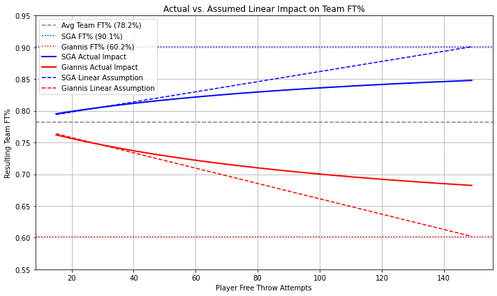
Realistically, these high volume shooters will take 30-50 free-throw attempts during a week of NBA matchups, but a team also has 13 players, each of whom only impacts their team’s overall percentage in the same, limited way. When compared to the linear assumption, we begin to answer the questions above paragraph: No, Giannis and Shae don’t help or hurt as much as they’re given credit for.
SHAW Percentage Transformation
It seems reasonable, then, that percentage transformations for fantasy rankings should be treated with this observation in mind. Attempts should be weighted within limits (defined by its distribution) to reflect the non-linearity of their effect on percentages.
I apply a Sigmoid-transformation to attempts to get a weight value. The Sigmoid transformation is defined as follows:
\[\text{Weight} = \left( \frac{S - 1}{0.5} \right) \left( \frac{1}{1 + e^{-k (x - 1)}} - 0.5 \right) + 1\]Where:
- x = Attempts / Average Attempts
- S = 1 + CoV (Coefficient of Variation)
- k = 1 / (1 + Skewness)
Applying to attempts in a percentage category, this yields weight values of 1 when a player’s attempts are at the league average, and a maximum of 1 + CoV (which for Free Throws is 2.17). For attempts below average, the player is assigned a weight value below one.
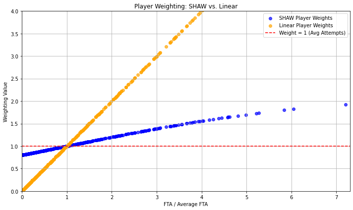
I then apply the weight directly to the percentage deficit, or difference from the mean, which I cap at 3 standard deviations from the mean, effectively limiting the impact that a few terrible shooters have on the rest of the distribution (Giannis is well within 3 standard deviations of the mean of simple percentage).
# Define Sigmoid Weight for Attempts
def sensitivity(attempts):
    return 1 + attempts.std() / attempts.mean() # 1 + CoV for maximum weight

def lambda_val(attempts):
    return 1 / (1 + abs(skew(attempts))) # 1 / 1 + skewness for modest slope

def sig_weight(attempts):

    avg_attempts = attempts.mean()
    # Ratio of attempts to average
    x = attempts / avg_attempts

    k = lambda_val(attempts)
    S = sensitivity(attempts)

    # Calculate the sigmoid transformation
    sigmoid = 1 / (1 + np.exp(-k * (x - 1)))

    # Scale and center the sigmoid function
    weight = ((S - 1) / 0.5) * (sigmoid - 0.5) + 1

    return weight

# Define function to transform a percentage stat
def SHAW_transform(nba, stat, attempts, makes):

    # League Average Percentage (using eligible (25+ GP) players)
    league_avg = nba[makes].sum() / nba[attempts].sum()

    # Deficit = percentage - average
    nba[f"{stat}_deficit"] = -(global_avg - nba[stat])

    # Clip extreme deficits to prevent outliers from dominating
    max_deficit = nba[f"{stat}_deficit"].std() * 3
    nba[f"{stat}_deficit"] = nba[f"{stat}_deficit"].clip(lower=-max_deficit, upper=max_deficit)

    # Weight = sigmoid transformed attempts
    nba[f"{stat}_weight"] = sig_weight(nba[attempts])

    # SHAW transformation = Deficit * Weight
    nba[f"SHAW_{stat}"] = nba[f"{stat}_deficit"] * nba[f"{stat}_weight"]

    # Finally, remove players not meeting minimum attempts threshold from the distribution (while keeping the rows)
    min_attempts = nba[attempts].quantile(minimum_attempts_quantile)
    nba.loc[stats[attempts] < min_attempts, f"SHAW_{stat}"] = np.nan

    return stats

# Apply transformation function to FT%, FG%, and 3P%
nba = SHAW_transform(nba, "FT_PCT", "FTA", "FTM")
nba = SHAW_transform(nba, "FG_PCT", "FGA", "FGM")
nba = SHAW_transform(nba, "FG3_PCT", "FG3A", "FG3M")

# so that 0 percents don't become nans
SHAW_percentages = ['SHAW_FT_PCT', 'SHAW_FG_PCT', 'SHAW_FG3_PCT']
for col in SHAW_percentages:
    nba[col] = nba[col].fillna(0)
The resulting distribution is the sigmoid-heuristic attempts-weighted deficit, which could be added back to a player’s raw percentage, or left alone, because the resulting dispersion is the same.
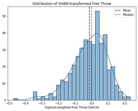
SHAW-transformed percentages appear to follow a reasonably normal distribution that can be appropriately scaled to compare to other cumulative categories. If standardizing, for example, the extreme values that were produced in the tails (Giannis vs. SGA for example) using Impact scores are now muted by SHAW-tranformations. Compared to existing methods, this method thus undervalues SGA and overvalues Giannis. It ammounts to a -2.2 point swing for SGA and + 4.6 point swing for Giannis in Z-score ranking systems, which is plenty enough to change their positions (except for the fact that SGA is a top 5 player anyway, he hardly moves).
Table: Standardized Free Throw Impact vs. Standardized SHAW-tranformed Free Throw Percentage
| Player Name | FT% | FTM | FTA | Attempts / Average | FT Impact Z Score | Deficit | Sig-weight | SHAW% | SHAW Z Score |
|---|---|---|---|---|---|---|---|---|---|
| Giannis Antetokounmpo | 60.2 | 369 | 613 | 5.59 | -8.12 | -0.18 | 1.65 | 48.6 | -3.55 |
| Steph Curry | 92.9 | 252 | 234 | 2.30 | 2.73 | 0.15 | 1.21 | 96.1 | 2.30 |
| Shae Gilgeous-Alexander | 90.1 | 563 | 625 | 5.70 | 5.50 | 0.12 | 1.66 | 98.0 | 2.52 |
| James Harden | 87.4 | 515 | 450 | 5.70 | 3.51 | 0.09 | 1.56 | 92.5 | 1.85 |
| LeBron James | 76.8 | 289 | 222 | 2.63 | -0.23 | -0.01 | 1.27 | 76.4 | -0.13 |
The empirical question is: Does the resulting difference (Impact vs. SHAW scaling) in overall rankings produce a more or less competitive team? Next I construct a series of unique ranking algorithms using the SHAW scaling method, to compare to traditional and industry rankings.
Standardization
Standardization works by transforming unique distributions to the same theoretical range (mean = 0 and standard deviation = 1) so that they can be easily compared. Again, a Z-score is found by taking a player’s difference from teh mean and dividing by the standard deviation.
In Python:
def Z(stat):
    return (stat - stat.mean())/stat.std()
I create a SHAW-Z ranking by including my SHAW-tranformed percentages in the set of categories to be standardized, taking the sum of those Z-Scores, and returning a rank-order.
nine_cat = ['SHAW_FT_PCT', 'SHAW_FG_PCT', 'PTS', 'FG3M', 'REB', 'AST', 'STL', 'BLK', 'tov']

def Z_rank(df, categories, metric_label):
    df[metric_label] = Z(df[categories]).sum(axis=1) # rank and add the categories
    df[metric_label + "_rank"] = df[metric_label].rank(ascending=False, method='min').reindex(df.index) # return rank order
    return df

pg_stats = Z_rank(pg_stats, nine_cat, 'SHAW-Z')
The only difference between my SHAW Z-ranking and Traditional Z-ranking is the way that the percentage categories are scaled. Seven of the nine comparable categories would have the same exact standardized values before summing.
Min-Max Scaling
Similar to standardization, Min-Max scaling (transforming the range to 0 – 1) preserves the spread, but it also limits the range, so outlier values are reigned in. This means that if a player is an outlier in a category, their maximum value in a category is limited at 1, and all other players are scaled accordingly. This makes intuitive sense, because each category is only worth 1 point. If a fantasy team over-performs in a category, they don’t get more than one point, so it may make some sense to limit a players’ overall contributions.
To scale between 0-1, take the difference from the minimum value and divide by the range:
x’ - min(X) / (max(X) - min(X))
Because this approach is standard for many machine learning tasks, the conventional method in Python makes use of the ML SciKitLearn library.
from sklearn.preprocessing import MinMaxScaler

# scaler = MinMaxScaler() # default range = 0-1
x' = scaler.fit_tranform(x)
I create a SHAW-mm ranking by including my SHAW-tranformed percentages in the set of categories to be scaled between 0 and 1, taking the sum of those Min-Max scores, and returning a rank-order.
def minmax_rank(df, categories, metric_label):
    scaler = MinMaxScaler() # default range = 0-1
    df[metric_label] = scaler.fit_transform(df[categories]).sum(axis=1) # rank and add the categories
    df[metric_label + "_rank"] = df[metric_label].rank(ascending=False, method='min').reindex(df.index) # return rank order
    return df

pg_stats = minmax_rank(pg_stats, nine_cat, 'SHAW-mm')
Scarcity Ranking
Scarcity is the basis of modern economics because scarce resources are more valuable than abundant ones (c.f., David Ricardo, 1817). In an NBA game, there are plenty of points scored and many players accumulate points. By contrast, blocked shots or steals might happen a handful of times in a game, and only a few players across the league tend to excel in those categories.
Although Blocks and Points count the same in terms of weekly scoring, having a player that excels in Blocks may be more valuable than a high Points-getter, because the Block star is harder to replace. There are fewer elite shot blockers in the league, and if your team doesn’t have one, you may have a hard time competing in that category.
To test this hypothesis, I developed an index that weighs the relative scarcity of each of the seven cumulative categories (on a scale of 0-1, total scarcity = 1) by subtracting the skew from the inner-quartile range, and normalizing (Min-Max scaling) the results. Then, for the Min-Max transformed categories, I multiply by its scarcity score. The result is a modest addition that boosts a player’s min-max score: the more proficient a player is in the more scarce categories, the bigger the boost. Although the boost is modest (the maximum boost is < 2 points (in a 9 x 1 category field of possibles)), it should be enough to empirically observe whether scarce category producers prove more valuable.
def scarcity_rank(df, categories, metric_label):

    # Calculate skewness and interquartile range for each category
    skewness = df[categories].apply(skew)
    iqr = df[categories].quantile(0.75) - df[categories].quantile(0.25)

    # Compute scarcity index (skewness / IQR) and scale it to [0, 1]
    scarcity_index = (skewness / iqr).sort_values(ascending=False)
    scarcity_weights = (scarcity_index - scarcity_index.min()) / (scarcity_index.max() - scarcity_index.min())

    scaler = MinMaxScaler()
    # Scale each category and apply scarcity weights
    for stat in categories:
        # Scale the category to a 0-1 range
        df[f'{stat}_mm'] = scaler.fit_transform(df[[stat]])

        # Apply the scarcity weight to the scaled category
        df[f'{stat}_mm_scarcity_weight'] = df[f'{stat}_mm'] * scarcity_weights[stat]

    # Sum the scarcity-weighted stats
    df[f'{metric_label}_scarcity_boost'] = df[[f'{stat}_mm_scarcity_weight' for stat in categories]].sum(axis=1)

    # Add the boost to the original min-max scaled metric
    df[f'{metric_label}_mm_total'] = df[[f'{stat}_mm' for stat in categories]].sum(axis=1)
    df[f'{metric_label}_scarcity_score'] = df[f'{metric_label}_mm_total'] + df[f'{metric_label}_scarcity_boost']

    # Rank based on the final scarcity score
    df[f'{metric_label}_scarcity_rank'] = df[f'{metric_label}_scarcity_score'].rank(ascending=False, method='min')

    return df

counting_stats = ['PTS', 'FG3M', 'REB', 'AST', 'STL', 'BLK', 'tov']

pg_stats = scarcity_rank(pg_stats, counting_stats, '9_cat')
Other Ranking Methods
Other plausible ranking methods use the SHAW transformed percentages but forgo additional transformations and concerns with category variance.
Ranked Sum of Category Ranks
The simplest method is to rank players in each category, add up those ranks, and reverse rank that sum.
def cat_rank_sum(df, categories, metric_label):
    category_ranks = pd.DataFrame()
    for stat in categories:
        cat_ranks[stat + "_rank"] = df[stat].rank(ascending=False, method='min')
    df[metric_label] = cat_ranks.sum(axis=1)
    df[metric_label + "_rank"] = df[metric_label].rank(ascending=True, method='min')
    return df

pg_stats = cat_rank_sum(pg_stats, nine_cat, 'SHAW_rank_sum')
This method does not preserve the relative spread, but instead distributes players uniformly in each category, while still accounting for the relative position of each player in each category. And since we’re comparing all the players across all categories, this method seems elegant. As we’ll see, however, it does not perform well.
Head to Head Individual Player Comparisons
Another approach to ranking involves observing how players match up head-to-head (H2H) against other players. After SHAW-transforming the percentages, players are compared against every other player in every category. This requires building a data frame with a row for each player combination. From there we can count the number of categories that each player wins versus each other, we can assign a matchup winner (for most categories won), and we can count the total categories, and total matchup wins against the field.
This takes considerable computing time, so it’s not a practical method to build into an ETL pipeline. For the sake of comparison, I do construct the rankings based on H2H matchup wins and H2H each category wins, and compare these to the other metrics.
For brevity, the code for this can be found in my GitHub repository.
The six different ranking methods produce a lot of similar rankings, but enough variation to be meaningfully different, so they can be compared to each other, and compared to ESPN, Yahoo, and Basketball Monster.
Select NBA players and their ranks across 10 ranking algorithms
| Player Name | Traditional Z rank | SHAW Z rank | SHAW mm rank | SHAW Scarce mm rank | SHAW rank-sum rank | SHAW H2H each rank | SHAW H2H most rank | ESPN | Yahoo | Basketball Monster |
|---|---|---|---|---|---|---|---|---|---|---|
| Nikola Jokic | 1 | 2 | 1 | 2 | 2 | 2 | 1 | 5 | 1 | 1 |
| Shai Gilgeous-Alexander | 1 | 3 | 3 | 3 | 1 | 1 | 2 | 1 | 3 | 2 |
| Victor Wembanyama | 3 | 1 | 2 | 1 | 3 | 3 | 3 | 111 | 2 | 3 |
| Karl Anthony-Towns | 5 | 7 | 7 | 8 | 4 | 4 | 4 | 6 | 4 | 6 |
| Steph Curry | 10 | 10 | 8 | 9 | 21 | 20 | 34 | 16 | 12 | 13 |
| James Harden | 16 | 17 | 17 | 15 | 14 | 15 | 10 | 12 | 27 | 19 |
| LeBron James | 21 | 23 | 22 | 19 | 19 | 19 | 13 | 17 | 14 | 21 |
| Giannis Antetokounmpo | 81 | 26 | 43 | 28 | 90 | 89 | 75 | 3 | 23 | 76 |
| Dyson Daniels | 31 | 30 | 72 | 47 | 92 | 92 | 76 | 51 | 31 | 15 |
The Competition
I mentioned earlier that there is no transparency as to how the major platforms compute rankings, and to be fair, Yahoo and ESPN’s fantasy player portals don’t actually include rank numbers after the season begins. Nevertheless, they do provide an ostensibly rank-ordered list that can be sorted based on season totals, per-game averages, two week averages, etc. Because the order changes based on the parameter, and because the top players are congruent with other rankings, it is reasonable to assume there is a ranking algorithm working behind the scenes. Still, it should probably be noted that the results that follow (which would be bad for ESPN and Yahoo) are attributable to lack of clarity around what their player lists actually represent.
ESPN provides a separate ‘updated category rankings’ list every week, but these are based on future projections – designed to help fantasy managers make replacement decisions - and they are different from the lists provided in their fantasy player portal. Still, it does appear that ESPN uses some type of forecast ranking system that accounts for injuries, even for their “season averages” list. Why Victor Wembanyama was listed by ESPN at the 111th position on their list, however, is a mystery. I would think he should either be a top 10 player by “season averages” measures, or he should be completely removed (for forecasting purposes) because he suffered a season-ending blood condition mid-way through the seaon. I also compare Basketball Monster’s rankings. BBM keeps a very clear ranking system that appears to be true to real “season averages”, and it does not deviate much from the traditional Z-Score rankings.
I copy/pasted the top 200 players from each of the above statistics on March 26, 2025. I mention the date because the following are single point-in-time comparison. I refreshed my own rankings on March 26, so that I’m comparing player rankings using the same player statistics.
There were several players in Yahoo’s and ESPN’s season-average rankings that were filtered out of my own player pool because they did not meet my own minimum games threshold. These include Joel Embiid, who has only played 19 games this season, and Daeqwon Plowden - a player whose playing time increased only towards the end of the season, and whom Yahoo mysteriously had ranked #16. Although these players had ranks elsewhere, they were not in the eligible player pool and thus were removed from rank comparisons.
Comparing Rankings Using Top-n Player Matchups
I compare rankings by simulating head-to-head, 9-category matchups using the top-n players in each ranking system.
The code below builds a set of summary dataframes: a dataframe for each top-n depth (e.g., top 20 players); with a row for each ranking metric (or team); and a column for each of the 9 comparable categories. ‘League’ participants (or ‘teams’) can include any number of ranking metrics, and any number and any depth of top-n teams. Matchups can include more or less categories, for those wanting to compare rankings for custom league settings.
# Variable 'League' participants
all_metrics = ['Traditional_Z_rank', 'ESPN rank', 'Yahoo rank', 'BBM rank', 'SHAW_AVG_rank',
               'SHAW_Z_rank', 'SHAW_mm_rank', 'SHAW_Scarce_mm_rank', 'SHAW_rank_sum_rank',
               'SHAW_H2H_each_rank', 'SHAW_H2H_most_rank']

# Variable 'Team' construction
top_n_list = [20, 50, 100, 130]

# Variable Scoring Format
comp_stats = ['FG_PCT', 'FT_PCT', 'PTS', 'FG3M', 'REB', 'AST', 'STL', 'BLK', 'tov']

# Put per-game summary stats in a DataFrame, calculating percentages as total Makes/Attempts
def generate_summary_dfs(df, rank_metrics, top_n_list, categories):
    """
    For each top-N value and ranking metric:
        - Select top N players
        - Sum team stats, compute shooting percentages

    Returns:
        - summary_dfs: dict of DataFrames with cumulative raw stats per metric per top-N
    """
    summary_dfs = {}

    for n in top_n_list:
        summary_stats = {}

        for metric in rank_metrics:
            top_players = df.sort_values(by=metric).head(n)

            # Sum makes and attempts
            FGM = top_players['FGM'].sum()
            FGA = top_players['FGA'].sum()
            FTM = top_players['FTM'].sum()
            FTA = top_players['FTA'].sum()

            # Calculate percentages
            FG_PCT = FGM / FGA if FGA > 0 else 0
            FT_PCT = FTM / FTA if FTA > 0 else 0

            # Sum counting stats
            total_stats = top_players[['PTS', 'FG3M', 'REB', 'AST', 'STL', 'BLK', 'tov']].sum()

            # Add derived stats
            total_stats['FG_PCT'] = FG_PCT
            total_stats['FT_PCT'] = FT_PCT

            summary_stats[metric] = total_stats

        # Convert to DataFrame
        summary_df = pd.DataFrame(summary_stats).T
        summary_dfs[f'top_{n}'] = summary_df

    return summary_dfs

# Compare stats in a separate function
def compare_summary_dfs(summary_dfs, categories):
    """
    Takes in summary_dfs and performs head-to-head matchups.
    Returns matchup results as a dictionary of Series showing win counts per metric.
    """
    matchup_results_by_top_n = {}

    for label, summary_df in summary_dfs.items():
        metrics = summary_df.index.tolist()

        # Add columns for storing results
        summary_df['Total_Category_Wins'] = 0
        summary_df['Total_Matchup_Wins'] = 0

        # Compare each metric against all others for Total_Category_Wins and Total_Matchup_Wins
        for i, m1 in enumerate(metrics):
            for m2 in metrics[i+1:]:
                team1 = summary_df.loc[m1]
                team2 = summary_df.loc[m2]

                m1_wins = 0
                m2_wins = 0

                for cat in categories:
                    if cat in summary_df.columns:
                        if team1[cat] > team2[cat]:
                            m1_wins += 1
                        elif team1[cat] < team2[cat]:
                            m2_wins += 1

                # Update total category wins
                summary_df.loc[m1, 'Total_Category_Wins'] += m1_wins
                summary_df.loc[m2, 'Total_Category_Wins'] += m2_wins

                # Update total matchup wins
                if m1_wins > m2_wins:
                    summary_df.loc[m1, 'Total_Matchup_Wins'] += 1
                elif m2_wins > m1_wins:
                    summary_df.loc[m2, 'Total_Matchup_Wins'] += 1
                else:
                    summary_df.loc[m1, 'Total_Matchup_Wins'] += 0.5
                    summary_df.loc[m2, 'Total_Matchup_Wins'] += 0.5

        matchup_results_by_top_n[label] = summary_df[['Total_Matchup_Wins', 'Total_Category_Wins']]

    return matchup_results_by_top_n


summary_dfs = generate_summary_dfs(
    df=pg_player_ranker,
    rank_metrics=all_metrics, # Variable League Composition
    top_n_list=top_n_list, # Variable Team Construction
    categories=comp_stats # Variable League Scoring Format
)

matchups = compare_summary_dfs(
    summary_dfs=summary_dfs,
    categories=comp_stats
)
From there, the matchups object can be analyzed to compare total matchup wins for each team, or total category wins.
for label, result in matchups.items():
    print(f"\n🏀 Head-to-head wins among metrics ({label}):")
    print(result)
At the outset, I showed the total matchup wins from a top-20 players comparison across rankings (excluding BBM). The SHAW Z ranking scored impressively well against other metrics, including the Traditional Z rankings, winning 7 out of 8 total matchups, compared to only four for the Traditional Z ranking, 3 for ESPN and 1 for Yahoo. A closer analysis muddies that picture quite a bit, however.
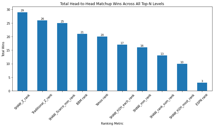
At deeper top-n’s, the results start to average out. Adding the results from across top 20, top 50, top 100, and top 130, in a 10 team league, for example, SHAW-Z rankings still win, but suddenly Traditional Z rankings perform much better than before, now beating rankings that beat it at the top 20 depth. This means that at the other levels - top 50, top 100, top 130 - Traditional Z rankings are actually winning more.
To illustrate this pattern with another example, when I put my six rankings in a league along with Basketball Monster rankings. Shaw Z rankings tie with BBM at the top 50 level, SHAW Z and SHAW-mm get the top two spots in the top 100 level, and BBM has the best overall top-130 player team in head to head matchups.
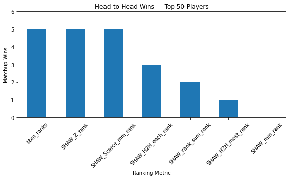
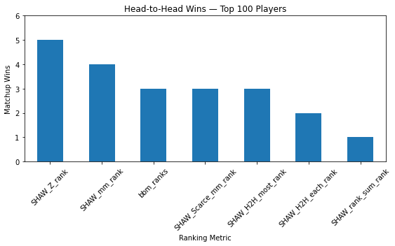
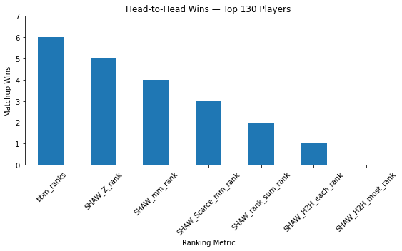
Three further complications:
- Different teams perform differently in relation to each other when league compositions change.
- There seems to be no stability in the depth that a particular ranking metric performs better or worse than others.
Watch what in a league that sums matchup wins for a.) the Top 10, 30, 50, 70, and 90 player teams, and compares those with the sum of matchup wins for b) the Top 20, 40, 60, 80, and top 100 teams.
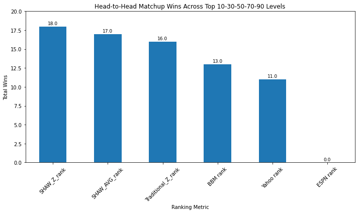
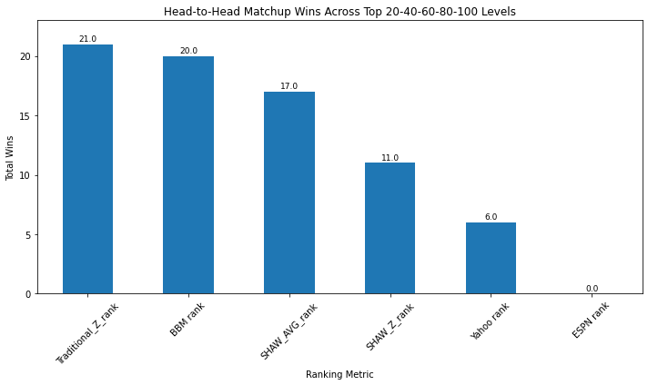
While SHAW Z wins most matchups for the first set, it places 4th in the next set. And overall, I have to admit, if adding all the matchup wins at each top-10 level for the first 100 players, Traditional Z scores wins more. When comparing the top 130 players (the number drafted in a 10 team league), the SHAW-AVG ranking narrowly beats all others.
Fortunately, there is some stability when comparing most category wins, as the results are roughly congruent with matchup wins for same teams in same leagues.
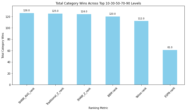
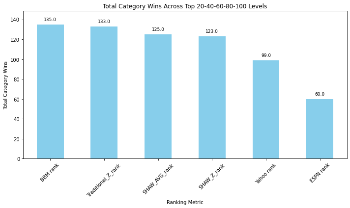
Many of my rankings outperformed the competition in head-to-head matchups. Specifically, my Z-ranking beat other rankings that are based on standardization in many of the matchups, which attests to the novel way that I treat percentage transformations. Additionally, the relative success of my ‘scarcity boosted’, Min-Max ranking should demonstrate that scarcity does matter, and this finding should inform future improvements.
Value over Replacement
I construct one final metric for my player-ranker dashboard, a VORP score – which I construct as the difference between a players SHAW Z score and the average SHAW Z score among players in the 100-150 range of the SHAW-AVG ranking list. This metric is essentially the same as a players SHAW Z score, minus a typical replacement’s average. Such a metric is useful for draft considerations when and if a manager needs to deviate from rank order for team-strategy or league position requirements - a potential player’s relative value difference from each other can be assessed.
pg_player_ranker = pg_stats.copy()

app_metrics = ['Traditional_Z_rank', 'SHAW_AVG_rank', 'SHAW_Z_rank', 'SHAW_mm_rank',
               'SHAW_Scarce_mm_rank', 'SHAW_rank_sum_rank',
               'SHAW_H2H_each_rank', 'SHAW_H2H_most_rank']

app_df = pg_player_ranker[['PLAYER_NAME'] + app_metrics + ['GP', 'FG_PCT', 'FT_PCT',
                        'PTS', 'FG3M', 'REB', 'AST', 'STL', 'BLK',
                        'FGM', 'FGA', 'FTM', 'FTA', 'TOV', 'tov'] + SHAW_percentages].copy()

# Define Replacement Value
nine_cats = ['PTS', 'FG3M', 'REB', 'AST', 'STL', 'BLK',
             'tov', 'SHAW_FT_PCT', 'SHAW_FG_PCT']

replacement_pool = app_df.sort_values('SHAW_AVG_rank').iloc[100:150]
replacement_avg = replacement_pool[nine_cats].mean()

# Calculate deltas for each player vs replacement
for cat in nine_cats:
    app_df[f'delta_{cat}'] = app_df[cat] - replacement_avg[cat]

# Z-Score Normalize Using SHAW-percentage transformations
SHAW_Z_cols = []
for cat in nine_cats:
    delta_col = f'delta_{cat}'
    z_col = f'z_{cat}'

    mean = app_df[delta_col].mean()
    std = app_df[delta_col].std()
    app_df[z_col] = (app_df[delta_col] - mean) / std

    SHAW_Z_cols.append(z_col)

app_df['SHAW_VORP'] = app_df[SHAW_Z_cols].sum(axis=1)

# Summary
replacement_summary = app_df[['PLAYER_NAME', 'SHAW_Z_rank', 'SHAW_VORP']] \
    .sort_values('SHAW_VORP', ascending=False)

print(replacement_summary.head(20))
                 PLAYER_NAME  SHAW_Z_rank  SHAW_VORP
410        Victor Wembanyama          1.0  15.176913
317             Nikola Jokić          2.0  14.495543
370  Shai Gilgeous-Alexander          3.0  12.474555
22             Anthony Davis          4.0  10.513017
405        Tyrese Haliburton          5.0   9.453085
278              Luka Dončić          6.0   9.321440
238       Karl-Anthony Towns          7.0   8.589270
195             Jayson Tatum          8.0   8.145027
407             Tyrese Maxey          9.0   8.024980
374            Stephen Curry         10.0   7.873836
87            Damian Lillard         11.0   7.736125
252             Kevin Durant         12.0   7.654458
268             Kyrie Irving         13.0   7.556756
263       Kristaps Porziņģis         14.0   7.358173
177             Jamal Murray         15.0   7.175387
23           Anthony Edwards         16.0   6.903803
179             James Harden         17.0   6.795028
127              Evan Mobley         18.0   6.777128
170            Jalen Johnson         19.0   6.706076
184        Jaren Jackson Jr.         20.0   6.622107
Streamlit User Endpoint
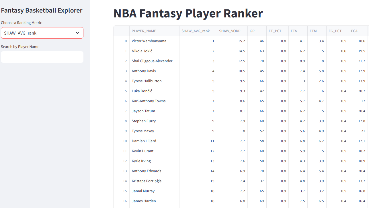
Finally, as a proof of concept, I build a Streamlit App as a user endpoint. The app allows the user to select among my top ranking metrics (except the H2H ones that take computing time). It is not yet deployed outside of my local drive, but my near-future goal is to make this publically accessible, executing the whole ETL pipeline described above.
import streamlit as st

# Set directory to where the script & CSV live
os.chdir("C:/Dat_Sci/Data Projects/NBA/Streamlit App")

# Page config
st.set_page_config(
    page_title="Fantasy Basketball Dashboard",
    layout="wide",
    initial_sidebar_state="expanded"
)

# Load data
app_df = pd.read_csv("ranking_app_df.csv")

# Sidebar setup
st.sidebar.title("Fantasy Basketball Explorer")

metric_options = ['SHAW_Z_rank', 'SHAW_mm_rank', 'SHAW_Scarce_mm_rank',
                  'SHAW_AVG_rank', 'SHAW_rank_sum', 'H2H_each_rank', 'H2H_most_rank']
selected_metric = st.sidebar.selectbox("Choose a Ranking Metric", metric_options)

# Stat columns to show
stat_columns = ["FT_PCT", "FTA", "FTM", "FG_PCT", "FGA", "FGM", "PTS",
                "FG3M", "REB", "AST", "STL", "BLK", "TOV"]
columns_to_show = ['PLAYER_NAME', selected_metric, 'SHAW_VORP', 'GP'] + stat_columns

# Sort and filter
df_display = app_df[columns_to_show].sort_values(selected_metric).reset_index(drop=True)


# Add player search bar
player_filter = st.sidebar.text_input("Search by Player Name")
if player_filter:
    df_display = df_display[df_display['PLAYER_NAME'].str.contains(player_filter, case=False)]

# Round
df_display = df_display.round(1)

# Title and display
st.title("NBA Fantasy Player Ranker")

st.dataframe(df_display, use_container_width=True, height=800)
Conclusions
On SHAW Transformations My SHAW percentage transformation rankings perform well, often (although not conclusively at every depth) beating other ranking algorithms, thus offering a competitive, statistically grounded ranking method. While the SHAW transformation is only a heuristic, the findings here support further analysis. Specifically, while my formulas for the sigmoid parameters, lambda and sensitivity, are based on properties of the attempts distributions (CoV & skewness), alternatives could be tested.
On Top-N Ranking Comparisons Regarding ranking comparisons, while I believe that this study is the first to offer any kind of systematic comparison, top n player comparisons might not be the best approach to evaluate ranking systems for at least two reasons. One reason is because there is inevitable overlap of players at every depth. If a ranking system fails by over penalizing a specific player at one level (e.g., Giannis is missing from the top 50 in Traditional Z Score rankings, despite that his production actually helps), for example, then that same ranking algorithm reintroduces that player in later depths (e.g., top 100), which gives that algorithm a huge boost for deeper matchups. Further, at the deepest levels, the rankings should basically exhaust all the relevant players, and thus they should all average out. In a 12-team fantasy league, 156 players will be drafted, which is actually more than the number of starting players in the NBA, so the top 156 by any ranking should either have tremendous overlap. And to the extent that are big differences between rankings at greater depths, it is probably safe to say that these’replacement-value’ players have a marginal impact anyway.
On Scarcity Value The criticism that Z scores over- or under-value outliers in skewed distributions is likely misguided. My standardized rankings beat the other SHAW rankings most of the time. Why? It turns out that standardization, like my scarcity boosted Min-Max ranking (which was very successful compared to the regular Min-Max scaled ranking), rewards scarcity. When a distribution is highly skewed, it is because the statistical event is relatively scarce, and/or because elite producers in that category are scarce. In fact, eliteness produces skew, and thus scarcity. Victor Wembanyama pushes out the tail of the distribution because he IS a unique talent; the skew results from the fact he alone does what others cannot. Wemby’s Z score of 8 in Blocks, or Dyson Daniel’s Z score of 6 in Steals not only reflect those player’s ability in relation to those categories, but they reflect their scarcity in relation to other players as well.
To say that standardization assumes a normal distribution may be like saying wearing running shoes assumes that I am running (Yes I am, and no I’m not). The form is not always the function. The misconception comes from the statistical concept of the central limit theorem, which allows us to assign probabilities to independent events occurring because of the fact that sample distributions ARE normally distributed when numbers are large. Then, standard deviations have real probabilities attatched. But we know that NBA stats aren’t normal, and we are not trying to test whether or not Wemby’s 3.5 Blocks per game comes from the same distribution as LeBron Jame’s 0.9 Blocks. We already know they do. We are, however, interested in knowing how Wembanyama’s 3.5 Blocks per game compares to Sabonis’ 14 Rebounds, or Trae Young’s 10+ Assists. Standardization simply gives us a like metric to compare categories that otherwise might have radically different ranges. The fact that it produces some astounding numbers at the tails in NBA stats is actually a benefit for comparing cumulative fantasy categories when the few players that can achieve those results can only be picked once.